Abstract
I report here on a successful attempt at reproducing the improvement in my ME/CFS symptoms that I usually experience during summer by means of artificially manipulating the temperature of the air, humidity, and the infrared radiation inside a room I spent five months in, during the period from December to April 2022. I show that the improvement is not correlated with the physical parameters of the air (temperature, relative and absolute humidity, atmospheric pressure, air density, dry air density, saturation vapor pressure, and partial vapor pressure). I hypothesize that it is driven instead by either the mid-wave infrared radiation emitted by a lamp used in the experiment or by the longwave infrared radiation emitted by the walls of the room in which I spent the months of the experiment.
1) Introduction
My ME/CFS improves during summer, in the period of the year that goes from May/June to the end of September (when I am in Rome, Italy). I don’t know why. In a previous study (Maccallini P. 2022), I analyzed the correlation between my symptoms and several environmental parameters, during three periods covering a total of 190 days: in one, I improved while the season was going toward summer, in another one we were in full-blown summer, and in the third one my functioning declined while summer was fading away. The statistical analysis showed a positive correlation between my functionality score and the temperature of the air and a negative correlation between my functionality score and air density and dry air density (remember that the higher the functionality score, the better I feel). No correlation was found between my functionality score and: relative humidity, absolute humidity, atmospheric pressure, and the concentration of particulate with a diameter below or equal to 
2) Methods
2.1) Data collection
I used a Bresser WiFi 4-in-1 Weather Station (see figure 1) to measure the temperature of the air, pressure, and relative humidity inside the room I spent almost all my time during the experiment. Measures were registered every 10 minutes and sent to the console which uploaded them to my Weathercloud account, via WiFi. The barometer was calibrated by using the closest weather station of the meteorological network of Rome (R). I registered a functionality score three times a day (value from 3 to 7, the higher the better) to use for the search for correlations with environmental data. The data that were employed were those of January, February, March, and April 2022. I also used the daily functionality score collected in 2017, during the same months, for testing the effect of the Summer Simulator on my symptoms.


Figure 1. Bresser 4-in-1 sensor: I used it to measure the temperature of the air, atmospheric pressure, and relative humidity inside the simulator. In the second image, you see the interface of the weather station (left) and a CO2 sensor I used to ensure that the air exchange in the room was adequate.
2.2) Summer Simulator
Simulation of summer was attempted with the following settings. I lived for 5 months in a room of 

To simulate thermal radiation, I used an infrared heater (Turbo TN35E, figure 3) coupled with a chamber with walls covered by mylar, a material that reflects most of the thermal radiation; the chamber was built around the bed, and it had only one side open, to allow for air circulation (figure 4).


Figure 4. The infrared chamber with walls made up of mylar, a material that reflects thermal radiation. On the right, you can see the heat pump (white) and the pipeline of the exhausted air, behind the curtain, that leads outside, through a hole in the window.
The infrared heater was, on average, at a distance of 0.8 m from the left side of the bed. It emits most of its power in the mid-wave infrared range (1-4 
2.3) Mathematical model for the infrared radiation
I built a mathematical model for the radiation from the lamp (Maccallini P. 2022) which predicts that the power per unit of area of a plane parallel to yz (see figure 4) centered in 
1) 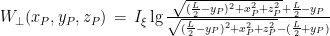
where L = 0.53 m is the length of the emitting surface of the lamp on the y axis and where
2) ![I_\xi\,=\,\frac{e\Pi(1-4b^2)\sqrt{1-4c^2}}{8\pi hLbc[F(\arctan\sqrt{\frac{1-4c^2}{4c^2}},\sqrt{\frac{1-4b^2}{1-4c^2}})-E(\arctan\sqrt{\frac{1-4c^2}{4c^2}},\sqrt{\frac{1-4b^2}{1-4c^2}})]}](https://s0.wp.com/latex.php?latex=I_%5Cxi%5C%2C%3D%5C%2C%5Cfrac%7Be%5CPi%281-4b%5E2%29%5Csqrt%7B1-4c%5E2%7D%7D%7B8%5Cpi+hLbc%5BF%28%5Carctan%5Csqrt%7B%5Cfrac%7B1-4c%5E2%7D%7B4c%5E2%7D%7D%2C%5Csqrt%7B%5Cfrac%7B1-4b%5E2%7D%7B1-4c%5E2%7D%7D%29-E%28%5Carctan%5Csqrt%7B%5Cfrac%7B1-4c%5E2%7D%7B4c%5E2%7D%7D%2C%5Csqrt%7B%5Cfrac%7B1-4b%5E2%7D%7B1-4c%5E2%7D%7D%29%5D%7D&bg=ffffff&fg=000000&s=0&c=20201002)
In this formula, e is the efficiency of the conversion of electrical power into mid-wave infrared emission (it is 93% according to the manufacturer) while 


Figure 5. On the left, the systems of coordinates used for building the mathematical model of the infrared heater. On the right, the detail of the ellipsoid that describes the concentration of the radiant power that exits the heater as a result of the power released by the bulb and the power reflected by the reflector behind the bulb; this ellipsoid is represented as a sphere on the left side of this figure. All the details of the model can be found in (Maccallini P. 2022).
The solution of the model (equations 1 and 2) was determined analytically, the values for the elliptic functions were calculated by employing Wolfram Mathematica 5.2 as a function of b and c and saved in a csv file, then the output of the lamp was calculated by a custom script written in Octave (Maccallini P. 2022) that used the output from the Mathematica script. Note that Octave does not have a built-in function for the elliptic functions and a numerical integration by Simpson’s rule led to unsatisfactory results, as detailed in the already mentioned reference. The prediction for a plane parallel to yz at a distance 

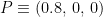


Figure 6. The power per unit of area orthogonal to the plane zy (
2.4) Derived environmental parameters
The weather station only measured air temperature, atmospheric pressure, and relative humidity, every 10 minutes. The measures were then uploaded via WiFi to a server and downloaded to my computer from my Weathercloud account. To calculate the daily means of these parameters I designed an algorithm that takes into account missing data, as follows: it calculates an hourly mean measure when at least one measure is available for that hour; it fills isolate missing hourly means with the mean between the measure of the hour before and the one of the following hour; it then calculates the daily mean if the hourly means of at least 21 hours are present for each day, otherwise the daily mean is considered as a missing value. From the hourly means of temperature, relative humidity, and pressure, I calculated the hourly means for saturation vapor pressure (SVP), partial vapor pressure (PVP), absolute humidity (AH), dry air density (DAD), and air density (AD), by means of the following formulae:
3) 
4)
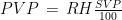
5)
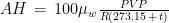
6)
7)

where t, p, RH are air temperature, barometric pressure, and relative humidity, respectively, while 

2.5) Statistical analysis
To assess the effect of the summer simulation on my symptoms, I compared the functionality score collected in 2017 (from January to April) with the score collected during the same months of 2022, while living inside the Summer Simulator. The null hypothesis was tested by running the Wilcox test. The correlations between the daily mean score and the environmental parameters were assessed by Spearman’s correlation coefficient and the significance of each correlation was also tested. All the calculations were performed by a custom R script written by myself, available, along with the row data, at the bottom of this page.
3) Results
The comparison between the mean daily scores for the months of January, February, March, and April 2017 and the same parameter for the same months of the year 2022 show that the Summer Simulator has raised the mean daily score in a statistically significant fashion: p value = 

Figure 7. Comparison between the mean daily functionality score in 2017 (from January to April), on the right, and the same score in 2022 (same months), while living inside the Summer Simulator, on the left. The difference is statistically significant, reaching a p value of


Figure 8. Daily mean values for each one of the environmental parameters considered in this study and for the functionality score, for the month of March.
The correlations between the mean daily score and the mean daily values of the environmental parameters, and the corresponding p values, are collected in Table 1. After correction for multiple comparisons (Benjamini-Hochberg method), none of the correlations reaches statistical significance.
| Parameter (daily mean) |  | p | p’ |
| Temperature | -0.2196 | 0.02059 | 0.1421 |
| Relative humidity | -0.1860 | 0.05068 | 0.1928 |
| Pressure | 0.05764 | 0.5497 | 0.5497 |
| Saturation vapor pressure | -0.2214 | 0.01955 | 0.1421 |
| Partial vapor pressure | -0.2081 | 0.02842 | 0.1421 |
| Absolute humidity | -0.2098 | 0.02711 | 0.1421 |
| Dry air density | 0.1686 | 0.07833 | 0.1928 |
| Air density | 0.1593 | 0.09641 | 0.1928 |
Table 1. Correlations between the mean daily functionality score and several environmental parameters (Spearman’s rank correlation coefficient) and the corresponding p values before and after correction for multiple comparisons (Benjamini-Hochberg method).
I run a similar analysis with another method, too: I compared the daily mean temperatures for days with a mean functionality score above 5 and the daily mean temperature for the days with a score below 5, by running the Wilcox test; I repeated this same analysis for all the other environmental parameters (see Table 2 and figure 8).


Figure 8. For each environmental parameter, you find here the comparison between the mean daily value corresponding to days with a mean functionality score above 5, equal to 5, and below 5. Box and whisker plots, with also the indication of the means, as red dots. The p values for the comparisons between days with a mean functionality score below 5 and above 5 are collected in table 2.
| Parameter | p | p‘ |
| Temperature | 0.02694 | 0.1813 |
| Relative humidity | 0.133 | 0.2112 |
| Pressure | 0.2112 | 0.2112 |
| Saturation vapor pressure | 0.02535 | 0.1813 |
| Partial vapor pressure | 0.06324 | 0.1897 |
| Absolute humidity | 0.06213 | 0.1897 |
| Dry air density | 0.03038 | 0.1813 |
| Air density | 0.03625 | 0.1813 |
Table 2. For each environmental parameter, I compared the daily mean value corresponding to days with a functionality score above 5, with the same value for days with a functionality score below 5 (Wilcox test) and I corrected for multiple comparisons (Benjamini-Hochberg method).
4) Discussion
Simulation of summer by raising the air temperature, absolute humidity, and infrared radiation did show to improve my symptoms when I compared my daily functionality score with the score collected for the same period of the year, but in 2017, while I was following another therapy that I judged mildly effective (figure 7). Yet, no correlation reached statistical significance between my functionality score and the environmental parameters that could be measured or derived (temperature, relative and absolute humidity, atmospheric pressure, saturation vapor pressure, partial vapor pressure, dry air density, air density). If we accept that the summer simulation has really improved my condition (i.e. if we rule out a placebo effect), we must admit that the improvement was due to either some combination of the aforementioned parameters or something else. The only other parameter I could exert my control on was infrared radiation by an infrared heater that delivered a power of about 
One possible explanation, to my understanding, for the results of this study, is then that the improvement was driven by some effect of the radiation from the lamp, either directly on my body or indirectly to some other parameter of the environment which in turn affected my biology. Importantly, the absence of correlation with air temperature, air density, and dry air density reported by the present study suggests that the significant correlations found in the previous study (Maccallini P. 2022) between my functionality score and the three mentioned parameters were driven by something else that correlates with temperature (which negatively correlates with air density and dry air density). We know that there is an almost linear positive correlation between the temperature of the air and longwave infrared radiation from the Earth into space (Koll DDB and Cronin TW 2018), while the emission of the surface of the Earth within a short distance from it must follow the Stefan-Boltzman law so that it is proportional to 


I can’t rule out a placebo effect of the Summer Simulator, even though it showed greater effectiveness than another therapy I was following in 2017, which I considered mildly effective. The difficulty of assessing the effectiveness of a treatment by a subjective score can hardly be overestimated. The identification of objective measures that can be routinely used to score the level of symptoms is of paramount importance for correlation studies like the present one.
5) Conclusions
By simulating summer during the months from January to April of 2022, I experienced an improvement in my symptoms similar to the one I usually experience during summer (although of a lesser magnitude). The simulation was achieved by increasing air temperature and absolute humidity, by using an infrared heater, and by living inside a chamber covered with mylar, a material that reflects most of the thermal radiation, so to avoid dispersion of the radiation from the heater. The improvement does not correlate with any of the parameters of the air (temperature, absolute and relative humidity, saturation vapor pressure, partial vapor pressure, density of the air, density of dry air, atmospheric pressure). One possible explanation for my improvement while living inside the Summer Simulator is that it was due to either the direct radiation from the heater (which is mid-wave infrared radiation) or the radiation from the walls heated by the lamp and the air. The latter radiation is far infrared radiation, the same radiation emitted by the Earth, which linearly correlates with air temperature and which might drive the improvements I experience during summer and the correlation between my functionality score and air temperature reported in a previous study.
6) Funding
This study was supported by those who donated to this website.
7) Supplementary material
The environmental measures and the symptom scores used for this study are available for download:
Score_control_Summer_Simulator.csv
The mathematical model of the infrared heater is available here for download. The script I wrote in R for the statistical analyses is the following one.
# file name: summer_simulator
#
# year: 2022
# month: 08
# day: 31
#
#-------------------------------------------------------------------------------
# We read the measures from Bresser Weather Station
#-------------------------------------------------------------------------------
#
# We set the names of the columns for the data.frames containing environmental data
#
cn<-c("Date","Tempin","Temp","Chill","Dewin","Dew","Heatin","Heat","Humin","Hum",
      "Wspdhi","Wspdavg","Wdiravg","Bar", "Rain", "Rainrate","Solarrad","Uvi")
#
# We read the environmental data
#
Jan_2022<-read.csv("Weathercloud Paolo WS 2022-01.csv", sep = ";", col.names = cn, header = T)
Feb_2022<-read.csv("Weathercloud Paolo WS 2022-02.csv", sep = ";", col.names = cn, header = T)
Mar_2022<-read.csv("Weathercloud Paolo WS 2022-03.csv", sep = ";", col.names = cn, header = T)
Apr_2022<-read.csv("Weathercloud Paolo WS 2022-04.csv", sep = ";", col.names = cn, header = T)
List_2022<-list(Jan_2022, Feb_2022, Mar_2022, Apr_2022)
#
# We set some parameters
#
mis<-3 # the highest number of missing hours accepted for a day
muw<-18.01528 # molecular weight of water (g/mol)
mud<-28.97 # molecular weight of dry air (g/mol)
R<-8.31 # universal constant of gasses (J/(K*mole))
month_name<-c("January", "February", "March", "April")
#
#-------------------------------------------------------------------------------
# We work on the score
#-------------------------------------------------------------------------------
#
# We set the names of the columns for the data.frame containing the score
#
cn<-c("Year","Month","Day","score_1","score_2","score_3")
#
# We read the scores
#
Score<-read.csv("Score_Summer_Simulator.csv", sep = ";", col.names = cn, header = T)
Score_control<-read.csv("Score_control_Summer_Simulator.csv", sep = ";", col.names = cn, header = T)
#
attach(Score)
#
ms<-c(rep(0,31*4))
#
# We calculate the daily mean score
#
for (d in 1:length(Year)) {
  if (is.na(score_1[d])==F&is.na(score_2[d])==F&is.na(score_3[d])==F) {
    ms[d]<-(score_1[d] + score_2[d] + score_3[d])/3
  } else ms[d]<-NA
}
#
attach(Score_control)
#
ms_c<-c(rep(0,length(Year)))
#
# We calculate the daily mean score
#
for (d in 1:length(Year)) {
  if (is.na(score_1[d])==F&is.na(score_2[d])==F&is.na(score_3[d])==F) {
    ms_c[d]<-(score_1[d] + score_2[d] + score_3[d])/3
  } else ms[d]<-NA
}
#
# We test the effect of the simulator
#
wilcox.test(ms, ms_c)
boxplot(ms, ms_c, ylab = "score", names = c("summer simulator","other"))
#
#-------------------------------------------------------------------------------
# We calculate mean values for temp (°C), relative humidity (%), and atmospheric
# pressure (hPa)
#-------------------------------------------------------------------------------
#
# We initialize the arrays that will contain the daily means of the environmental
# data
#
t<-c(rep(0,31*4))
rh<-c(rep(0,31*4))
p<-c(rep(0,31*4))
svp<-c(rep(0,31*4))
pvp<-c(rep(0,31*4))
ah<-c(rep(0,31*4))
dad<-c(rep(0,31*4))
ad<-c(rep(0,31*4))
#
#-------------------------------------------------------------------------------
# We work on each month
#-------------------------------------------------------------------------------
#
for (q in 1:4) {
  index<-q
  add<-31*(q-1)
  attach(List_2022[[q]])
  #
  # We extract the day of the month, the year, the hour from column Date
  #
  DateR<-read.table(text=Jan_2022[,1], sep ="/")
  DateR2<-read.table(text=DateR[,3], sep =" ")
  DateR3<-read.table(text=DateR2[,2], sep =":")
  #
  #-------------------------------------------------------------------------------
  #
  first_day<-DateR[1,1]
  last_day<-DateR[length(DateR[,1]),1]
  #
  # We calculate the hourly mean for temperature (°C)
  #
  Temp_mean<-matrix(data=c(rep(0,31*24)), nrow = 31, ncol = 24)
  num<-matrix(data=c(rep(0,31*24)), nrow = 31, ncol = 24)
  #
  for (d in first_day:last_day) {
    for (h in 1:24) {
      for (j in 1:length(DateR[,1])) {
        if ( DateR[j,1]==d & DateR3[j,1]== h-1) {
          if (is.na(Temp[j])==F) {
            Temp_mean[d,h]<-(Temp_mean[d,h] + Temp[j])
            num[d,h]<-(num[d,h]+1)
          }
        }
      }
    }
  }
  for (d in first_day:last_day) {
    for (h in 1:24) {
      if (num[d,h]>0) Temp_mean[d,h]<-Temp_mean[d,h]/num[d,h] else Temp_mean[d,h]<-NA
    }
  }
  #
  # We fill isolate missing values
  #
  for (d in first_day:last_day) {
    for (h in 2:23) {
      if (is.na(Temp_mean[d,(h-1)])==F&is.na(Temp_mean[d,h])==T&is.na(Temp_mean[d,(h-1)])==F) {
        Temp_mean[d,h]<-(Temp_mean[d,(h-1)]+Temp_mean[d,(h+1)])/2
      }
    }
  }
  for (d in (first_day+1):(last_day-1)) {
    if (is.na(Temp_mean[(d-1),(24)])==F&is.na(Temp_mean[d,1])==T&is.na(Temp_mean[d,2])==F) {
      Temp_mean[d,1]<-(Temp_mean[(d-1),24]+Temp_mean[d,2])/2
    }
  }
  #
  # We calculate the daily mean for temperature (°C)
  #
  for (d in first_day:last_day) {
    count<-0
    for (h in 1:24) {
      if (is.na(Temp_mean[d,h])==T) count<-count+1
    }
    if (count<=mis) t[add+d]<-mean(Temp_mean[d,],na.rm = T) else t[add+d]<-NA
  }
  #
  # We calculate the hourly mean relative humidity (%)
  #
  RH_mean<-matrix(data=c(rep(0,31*24)), nrow = 31, ncol = 24)
  num<-matrix(data=c(rep(0,31*24)), nrow = 31, ncol = 24)
  #
  for (d in first_day:last_day) {
    for (h in 1:24) {
      for (j in 1:length(DateR[,1])) {
        if ( DateR[j,1]==d & DateR3[j,1]== h-1) {
          if (is.na(Hum[j])==F) {
            RH_mean[d,h]<-(RH_mean[d,h] + Hum[j])
            num[d,h]<-(num[d,h]+1)
          }
        }
      }
    }
  }
  for (d in first_day:last_day) {
    for (h in 1:24) {
      if (num[d,h]>0) RH_mean[d,h]<-RH_mean[d,h]/num[d,h] else RH_mean[d,h]<-NA
    }
  }
  #
  # We fill isolate missing values
  #
  for (d in first_day:last_day) {
    for (h in 2:23) {
      if (is.na(RH_mean[d,(h-1)])==F&is.na(RH_mean[d,h])==T&is.na(RH_mean[d,(h-1)])==F) {
        RH_mean[d,h]<-(RH_mean[d,(h-1)]+RH_mean[d,(h+1)])/2
      }
    }
  }
  for (d in (first_day+1):(last_day-1)) {
    if (is.na(RH_mean[(d-1),(24)])==F&is.na(RH_mean[d,1])==T&is.na(RH_mean[d,2])==F) {
      RH_mean[d,1]<-(RH_mean[(d-1),24]+RH_mean[d,2])/2
    }
  }
  #
  # We calculate the daily mean relative humidity (%)
  #
  for (d in first_day:last_day) {
    count<-0
    for (h in 1:24) {
      if (is.na(RH_mean[d,h])==T) count<-count+1
    }
    if (count<=mis) rh[add+d]<-mean(RH_mean[d,],na.rm = T) else rh[add+d]<-NA
  }
  #
  # We calculate the hourly mean pressure (hPa)
  #
  P_mean<-matrix(data=c(rep(0,31*24)), nrow = 31, ncol = 24)
  num<-matrix(data=c(rep(0,31*24)), nrow = 31, ncol = 24)
  #
  for (d in first_day:last_day) {
    for (h in 1:24) {
      for (j in 1:length(DateR[,1])) {
        if ( DateR[j,1]==d & DateR3[j,1]== h-1) {
          if (is.na(Hum[j])==F) {
            P_mean[d,h]<-(P_mean[d,h] + Bar[j])
            num[d,h]<-(num[d,h]+1)
          }
        }
      }
    }
  }
  for (d in first_day:last_day) {
    for (h in 1:24) {
      if (num[d,h]>0) P_mean[d,h]<-P_mean[d,h]/num[d,h] else P_mean[d,h]<-NA
    }
  }
  #
  # We fill isolate missing values
  #
  for (d in first_day:last_day) {
    for (h in 2:23) {
      if (is.na(P_mean[d,(h-1)])==F&is.na(P_mean[d,h])==T&is.na(P_mean[d,(h-1)])==F) {
        P_mean[d,h]<-(P_mean[d,(h-1)]+P_mean[d,(h+1)])/2
      }
    }
  }
  for (d in (first_day+1):(last_day-1)) {
    if (is.na(P_mean[(d-1),(24)])==F&is.na(P_mean[d,1])==T&is.na(P_mean[d,2])==F) {
      P_mean[d,1]<-(P_mean[(d-1),24]+P_mean[d,2])/2
    }
  }
  #
  # We calculate the daily mean pressure (hPa)
  #
  for (d in first_day:last_day) {
    count<-0
    for (h in 1:24) {
      if (is.na(P_mean[d,h])==T) count<-count+1
    }
    if (count<=mis) p[add+d]<-mean(P_mean[d,],na.rm = T) else p[add+d]<-NA
  }
  #
  # We calculate hourly mean saturation vapor pressure (hPa)
  #
  Svp_mean<-matrix(data=c(rep(0,31*24)), nrow = 31, ncol = 24)
  #
  for (d in first_day:last_day) {
    for (h in 1:24) {
      if (is.na(Temp_mean[d,h])==F) {
        Svp_mean[d,h]<-6.112*exp((17.62*Temp_mean[d,h])/(243.12 + Temp_mean[d,h]))
      } else Svp_mean[d,h]<-NA
    }
  }
  #
  # We calculate daily mean saturation vapor pressure (hPa)
  #
  for (d in first_day:last_day) {
    count<-0
    for (h in 1:24) {
      if (is.na(Svp_mean[d,h])==T) count<-count+1
    }
    if (count<=mis) svp[add+d]<-mean(Svp_mean[d,],na.rm = T) else svp[add+d]<-NA
  }
  #
  # We calculate hourly partial vapor pressure (hPa)
  #
  Pvp_mean<-matrix(data=c(rep(0,31*24)), nrow = 31, ncol = 24)
  #
  for (d in first_day:last_day) {
    for (h in 1:24) {
      if (is.na(Svp_mean[d,h])==F&is.na(RH_mean[d,h])==F) {
        Pvp_mean[d,h]<-RH_mean[d,h]*Svp_mean[d,h]/100
      } else Pvp_mean[d,h]<-NA
    }
  }
  #
  # We calculate daily mean partial vapor pressure (hPa)
  #
  for (d in first_day:last_day) {
    count<-0
    for (h in 1:24) {
      if (is.na(Pvp_mean[d,h])==T) count<-count+1
    }
    if (count<=mis) pvp[add+d]<-mean(Pvp_mean[d,],na.rm = T) else pvp[add+d]<-NA
  }
  #
  # We calculate hourly absolute humidity (g/m^3)
  #
  AH_mean<-matrix(data=c(rep(0,31*24)), nrow = 31, ncol = 24)
  #
  for (d in first_day:last_day) {
    for (h in 1:24) {
      if (is.na(Pvp_mean[d,h])==F&is.na(Temp_mean[d,h])==F) {
        AH_mean[d,h]<-100*Pvp_mean[d,h]*muw/( R*(273.15 + Temp_mean[d,h]) )
      } else AH_mean[d,h]<-NA
    }
  }
  #
  # We calculate daily mean absolute humidity (g/m^3)
  #
  for (d in first_day:last_day) {
    count<-0
    for (h in 1:24) {
      if (is.na(AH_mean[d,h])==T) count<-count+1
    }
    if (count<=mis) ah[add+d]<-mean(AH_mean[d,],na.rm = T) else ah[add+d]<-NA
  }
  #
  # We calculate hourly mean dry air density (g/m^3)
  #
  DAD_mean<-matrix(data=c(rep(0,31*24)), nrow = 31, ncol = 24)
  #
  for (d in first_day:last_day) {
    for (h in 1:24) {
      if (is.na(Pvp_mean[d,h])==F&is.na(Temp_mean[d,h])==F&is.na(P_mean[d,h])==F) {
        DAD_mean[d,h]<-100*(P_mean[d,h]-Pvp_mean[d,h])*mud/( R*(273.15 + Temp_mean[d,h]) )
      } else DAD_mean[d,h]<-NA
    }
  }
  #
  # We calculate daily mean dry air density (g/m^3)
  #
  for (d in first_day:last_day) {
    count<-0
    for (h in 1:24) {
      if (is.na(DAD_mean[d,h])==T) count<-count+1
    }
    if (count<=mis) dad[add+d]<-mean(DAD_mean[d,],na.rm = T) else dad[add+d]<-NA
  }
  #
  # We calculate hourly mean air density (g/m^3)
  #
  AD_mean<-matrix(data=c(rep(0,31*24)), nrow = 31, ncol = 24)
  #
  for (d in first_day:last_day) {
    for (h in 1:24) {
      if (is.na(DAD_mean[d,h])==F&is.na(AH_mean[d,h])==F&is.na(P_mean[d,h])==F) {
        AD_mean[d,h]<-AH_mean[d,h] + DAD_mean[d,h]
      } else AD_mean[d,h]<-NA
    }
  }
  #
  # We calculate daily mean dry air density (g/m^3)
  #
  for (d in first_day:last_day) {
    count<-0
    for (h in 1:24) {
      if (is.na(AD_mean[d,h])==T) count<-count+1
    }
    if (count<=mis) ad[add+d]<-mean(AD_mean[d,],na.rm = T) else ad[add+d]<-NA
  }
  #
  # We set as NA the days without measures, building arrays of 31 days
  #
  for (d in 1:31) if (d<first_day | d>last_day) {
    t[add+d]<-NA
    rh[add+d]<-NA
    p[add+d]<-NA
    svp[add+d]<-NA
    pvp[add+d]<-NA
    ah[add+d]<-NA
    dad[add+d]<-NA
    ad[add+d]<-NA
  }
  #
  # We plot mean temperature, relative humidity, pressure, saturation vapor pressure
  #
  plot (c((add+1):(add+31)),t[(add+1):(add+31)], type = "b", main =
          month_name[index], xlab = "day", ylab = "temperature (°C)", pch = 19,
        lty = 2, col = "red")
  grid(col="darkgray")
  plot (c((add+1):(add+31)),rh[(add+1):(add+31)], type = "b", main =
          month_name[index], xlab = "day", ylab = "relative humidity (%)", pch = 19,
        lty = 2, col = "red")
  grid(col="darkgray")
  plot (c((add+1):(add+31)),p[(add+1):(add+31)], type = "b", main =
          month_name[index], xlab = "day", ylab = "atmospheric pressure (hPa)", pch = 19,
        lty = 2, col = "red")
  grid(col="darkgray")
  plot (c((add+1):(add+31)),svp[(add+1):(add+31)], type = "b", main =
          month_name[index], xlab = "day", ylab = "saturation vapor pressure (hPa)", pch = 19,
        lty = 2, col = "red")
  grid(col="darkgray")
  plot (c((add+1):(add+31)),pvp[(add+1):(add+31)], type = "b", main =
          month_name[index], xlab = "day", ylab = "partial vapor pressure (hPa)", pch = 19,
        lty = 2, col = "red")
  grid(col="darkgray")
  plot (c((add+1):(add+31)),ah[(add+1):(add+31)], type = "b", main =
          month_name[index], xlab = "day", ylab = "absolute humidity (g/m^3)", pch = 19,
        lty = 2, col = "red")
  grid(col="darkgray")
  plot (c((add+1):(add+31)),dad[(add+1):(add+31)], type = "b", main =
          month_name[index], xlab = "day", ylab = "dry air density (g/m^3)", pch = 19,
        lty = 2, col = "red")
  grid(col="darkgray")
  plot (c((add+1):(add+31)),ad[(add+1):(add+31)], type = "b", main =
          month_name[index], xlab = "day", ylab = "air density (g/m^3)", pch = 19,
        lty = 2, col = "red")
  grid(col="darkgray")
  #
}
#
#-------------------------------------------------------------------------------
# We build a data frame that contains all the data of this study
#-------------------------------------------------------------------------------
#
attach(Score)
mydata<-data.frame(year = Year, month = Month, day = Day,
                   temperature = t, relative_hum = rh, pres = p, sat_vap_p = svp,
                   par_vap_p = pvp, absolute_hum = ah, dry_air_d = dad, air_d = ad,
                   score = ms)
attach(mydata)
#
#-------------------------------------------------------------------------------
# Spearman's correlation ranks
#-------------------------------------------------------------------------------
#
correlations<-list()
correlations[[1]]<-cor.test(score, temperature, alternative = "two.sided", method = "spearman",
         exact = T, conf.level = 0.95, continuity = T)
correlations[[2]]<-cor.test(score, relative_hum, alternative = "two.sided", method = "spearman",
         exact = T, conf.level = 0.95, continuity = T)
correlations[[3]]<-cor.test(score, pres, alternative = "two.sided", method = "spearman",
         exact = T, conf.level = 0.95, continuity = T)
correlations[[4]]<-cor.test(score, sat_vap_p, alternative = "two.sided", method = "spearman",
         exact = T, conf.level = 0.95, continuity = T)
correlations[[5]]<-cor.test(score, par_vap_p, alternative = "two.sided", method = "spearman",
         exact = T, conf.level = 0.95, continuity = T)
correlations[[6]]<-cor.test(score, absolute_hum, alternative = "two.sided", method = "spearman",
         exact = T, conf.level = 0.95, continuity = T)
correlations[[7]]<-cor.test(score, dry_air_d, alternative = "two.sided", method = "spearman",
         exact = T, conf.level = 0.95, continuity = T)
correlations[[8]]<-cor.test(score, air_d, alternative = "two.sided", method = "spearman",
         exact = T, conf.level = 0.95, continuity = T)
correlations[[9]]<-cor.test(temperature, air_d, alternative = "two.sided", method = "spearman",
         exact = T, conf.level = 0.95, continuity = T)
correlations[[10]]<-cor.test(temperature, dry_air_d, alternative = "two.sided", method = "spearman",
         exact = T, conf.level = 0.95, continuity = T)
#
#-------------------------------------------------------------------------------
# We search for the optimal environmental parameters
#-------------------------------------------------------------------------------
#
low_score<-subset.data.frame(mydata, score<5)
mean_score<-subset.data.frame(mydata, score==5)
high_score<-subset.data.frame(mydata, score>5)
#
# Hypotheses testing
#
# temperature
wilcox.test(low_score[,4], high_score[,4])
# relative humidity
wilcox.test(low_score[,5], high_score[,5])
# atm. pressure
wilcox.test(low_score[,6], high_score[,6])
# saturation vapor pressure
wilcox.test(low_score[,7], high_score[,7])
# partial vapor pressure
wilcox.test(low_score[,8], high_score[,8])
# absolute humidity
wilcox.test(low_score[,9], high_score[,9])
# dry air density
wilcox.test(low_score[,10], high_score[,10])
# air density
wilcox.test(low_score[,11], high_score[,11])
#
# Plotting
#
labels = c("temperature (°C)", "relative humidity (%)", "atm. pressure (hPa)",
           "saturation vapor pressure (hPa)", "partial vapor pressure (hPa)",
           "absolute humidity (g/m^3)", "dry air density (g/m^3)", "air density (g/m^3)")
for (i in 4:11) {
  boxplot(low_score[,i], mean_score[,i], high_score[,i], ylab = labels[i-3], names =
            c("score < 5", "score = 5", "score > 5") )
  points(1:3, c(mean(low_score[,i], na.rm = T), mean(mean_score[,i], na.rm = T),
                mean(high_score[,i], na.rm = T)), col = "red", pch = 18)
  grid(col="darkgray")
}
#
#-------------------------------------------------------------------------------
# We plot the mean score for each month
#-------------------------------------------------------------------------------
#
for (i in 1:4) {
  score_month<-subset.data.frame(mydata, month == i)
  plot (c(1:31),score_month[,12], type = "b", main =
          month_name[i], xlab = "day", ylab = "score", pch = 19,
        lty = 2, col = "red")
  grid(col="darkgray")
}

Grazie.
LikeLiked by 1 person
Veramente interessante! Chissà se i pannelli a infrarossi per riscaldamento domestico (quelli piatti e solitamente bianchi, ma anche colorati) possano produrre un effetto simile?
LikeLike