Whole Genome Sequencing was performed on the proband (me!) and three healthy family members: one paternal uncle and two maternal aunts. First-degree relatives were not available. Paired-FASTQ files were inputted to a GATK pipeline, according to GATK best practices workflows (R). After the generation of unmapped BAM from paired-FASTQ, a BAM file was obtained for each participant. The four GRCh38 BAM files were then submitted to joint variant calling along with other 50 genomes from the 1000 Genomes Project, used to maximize the signal/noise ratio. These analyses were all performed on the NHGRI AnVIL platform that offers virtual machines with optimized GATK configuration.
The resulting gVCF was submitted to Seqr for family filtering. Family filtering based on a dominant pattern of inheritance was performed with a threshold of zero for both QUAL and allele balance (quality filtering is performed in a following step). The result was downloaded and submitted to a custom R script (reported at the end of this page). The script filters out variants harbored by genes with a probability of being dominant below 0.5 (DOMINO score); it also eliminates calls with QUAL below 30. It then collects the remaining calls in a VCF file for submission to CADD GRCh38 v1.7 (R). The file containing the scores is then inputted again to the script that adds them to the Seqr output. Filtering is then performed as follows: the script retains only calls with CADD≥22.8, Eigen≥0, PolyPhen≥0.45, and SIFT≤0.05. Filtering is performed only when scores are available: so, for instance, a call with no available scores is kept.
Table. Results of Seqr permissive De Novo Dominant search on WGS, after filtering performed by my R script (see below). In the WES column: NA indicates that the variant is not present in the VCF file of WES, which can be due either to the fact that the position was not genotyped or to the fact that it was found homozygous for the reference allele; Y indicates that the position is present in WES with the same genotype. Same for 23&ME.
This pipeline selects four variants (see table). Two of them are present in a whole-exome performed on the proband, too. The other two are not present on WES and since only the VCF file is available for WES, we cannot say if they are absent because they were not genotyped or because the proband is homozygous for the reference allele. I then used reactome.org to select for each gene the pathway where its protein is involved in the higher number of reactions. Only CIC was not included in any pathway by Reactome, but it has been recently reported the involvement of CIC in folate transport into the brain and a few rare mutations in this gene have been proposed as causative for cerebral folate deficiency (R). None of the variants of the table has been associated with known diseases. The mitochondrial chromosome was analyzed by a custom R script, as detailed elsewhere (R), and nothing relevant was found. I’m currently performing further studies on these results and I am analyzing the structural variants of the proband.
# file name: Seqr_Dominant
#
# Rome 09th December 2023
#
#-------------------------------------------------------------------------------
# This script filters the results of Seqr's De Novo/Dominant Restrictive search
#-------------------------------------------------------------------------------
#
#-------------------------------------------------------------------------------
# Thresholds
#-------------------------------------------------------------------------------
#
co_CADD<-22.8 # a CADD phred score below co_CADD is considered tolerated
co_Eigen<-0 # a Eigen score below co_EIGEN is considered tolerated
co_PolyPhen<-0.45 # a PolyPhen score below co_PolyPhen is considered tolerated
co_SIFT<-0.05 # a SIFT score ABOVE co_SIFT is considered tolerated
#
PAD<-0.5 # Cut-off for probability of being Autosomal Disease (PAD)
#
co_Qual<-30 # threshold for quality score
#
#-------------------------------------------------------------------------------
# This function adds the probability of being a dominant gene
#-------------------------------------------------------------------------------
#
DOMINO<-function(variants) {
  #
  # Read the genes with their relative Domino probabilities
  #
  genes<-read.csv(file="C:/Users/macpa/OneDrive/Appunti/Genetics/Domino/DOMINO_GENEID_feb_2019.txt",sep="\t")
  colnames(genes)<-c("SYMBOL","gene","Domino")
  #
  # For each variant assign the DOMINO score of its gene (if any)
  #
  string<-"SYMBOL"
  if (substr(variants$gene[1],1,4)=="ENSG") string<-"gene"
  variants<-merge(variants,genes,by=string,all.x=T)
}
#
#-------------------------------------------------------------------------------
# This function generates a VCF file for CADD submission
#-------------------------------------------------------------------------------
#
VCF<-function(variants) {
  #
  variants<-variants[,2:5]
  variants$id<-rep(".",length(variants[,1]))
  temporary<-c("chrom","pos","id","ref","alt")
  variants<-variants[,temporary]
  write.table(variants,file="DeNovoDominant_permissive.vcf",quote=F,
              row.names=F,col.names=F,sep="\t")
}
#
#-------------------------------------------------------------------------------
# Read the seqr file and assign the domino probability
#-------------------------------------------------------------------------------
#
seqr_dom<-read.csv(file="DeNovoDominant_permissive.tsv", sep="\t", header = TRUE)
#
seqr_dom<-DOMINO(seqr_dom)
#
#-------------------------------------------------------------------------------
# Remove variants based on their Domino probability and quality
#-------------------------------------------------------------------------------
#
seqr_dom<-subset.data.frame(seqr_dom, Domino>=PAD | is.na(Domino)==T )
#
seqr_dom<-subset.data.frame(seqr_dom, gq_1>=co_Qual)
#
#-------------------------------------------------------------------------------
# Write file for CADD submission
#-------------------------------------------------------------------------------
#
VCF(seqr_dom)
#
#-------------------------------------------------------------------------------
# Read file after CADD submission
#-------------------------------------------------------------------------------
#
f.name<-gzfile("DeNovoDominant_permissive_CADD.tsv.gz")
CADDed<-read.csv(file=f.name,sep="\t",skip=1,comment.char=" ")
colnames(CADDed)<-c("chrom","pos","ref","alt","rawscore","cadd")
#
#-------------------------------------------------------------------------------
# Add cadd score
#-------------------------------------------------------------------------------
#
seqr_dom<-merge(seqr_dom,CADDed,by=c("chrom","pos","ref","alt"),all.x=T)
#
#-------------------------------------------------------------------------------
# Remove variants based on their in silico scores
#-------------------------------------------------------------------------------
#
seqr_dom<-subset.data.frame(seqr_dom, cadd.y>=co_CADD | is.na(cadd.y)==T )
seqr_dom<-subset.data.frame(seqr_dom, eigen>=co_Eigen | is.na(eigen)==T )
seqr_dom<-subset.data.frame(seqr_dom, polyphen>=co_PolyPhen | is.na(polyphen)==T )
seqr_dom<-subset.data.frame(seqr_dom, sift<=co_SIFT | is.na(sift)==T )
#
#-------------------------------------------------------------------------------
# Write output
#-------------------------------------------------------------------------------
#
write.table(seqr_dom,file="DeNovoDominant_permissive_filt.tsv",quote=F,row.names=F,col.names=T,sep="\t")
The distribution of age at diagnosis for ME/CFS patients follows a bimodal density, i.e. a density with two local maxima (Figure 1), according to the data collected from the Norwegian Patient Register from 2008 to 2012. Data were gathered considering the first G93.3 episode for each patient, and age was calculated as age in 2008 [Bakken IJ et al. 2014]. Code G93.3 is the ICD-10 label for postviral fatigue syndrome/benign myalgic encephalomyelitis. The sample size is 5809.
Univariate bimodal distributions can arise when the same variable is measured among two distinct populations: the classic example is human height, which displays a bimodal distribution because of the sexual dimorphism in our species (Figure 2). Bimodality can also be a consequence of selection bias [Finstad AG et al. 2004].
In the case of age at diagnosis of ME/CFS, one possible source of bimodality might be the presence of two different pathologies, one more prevalent among young individuals, with a mean age at diagnosis of 16-17 years, another more common among older individuals, with a mean age at diagnosis of about 40 years (Table 1, Table 2). The density of the two populations was derived by maximum likelihood estimation (MLE) performed by function mixfit() of the R package mixR [You Y 2021], after translation of Figure 1 of [Bakken IJ et al. 2014] into numeric data using WebPlotDigitizer [Aydin O et al. 2022]. The script that generates Figure 2, Table 1, and Table 2 is available at the end of this article.
Another possible explanation for the two-peak density of age at diagnosis might be a reduced susceptibility to ME/CFS during the third decade of life. Consistent with both these scenarios, a different prognosis for pediatric and adult ME/CFS patients has been documented, with 68% of the pediatric group reporting recovery by 10 years [Rowe KS 2019], while only 2% among adult patients experiences a progressive improvement [Stoothoff J et al. 2017].
Group
mean age
SD
alpha
lambda
Younger females (30%)
16.2
4.86
11.1
14.4
Older females
40.0
10.54
14.4
0.360
Younger males (35%)
17.5
4.76
8.6
0.493
Older males
47.6
13.42
12.6
0.264
Younger, overall (30%)
16.2
4.92
10.8
0.668
Older, overall
41.6
12.06
11.9
0.286
Table 1. Bimodal gamma fit performed by the function mixfit() of R package mixR [You Y 2021]. For each density, the mean and the standard deviation are indicated.The parameters alpha and lambda of the respective gamma densities are also collected.
Figure 1. Observed cases of ME/CFS by sex and one-year age group collected in the Norwegian Patient Register from 2008 to 2012. Age in 2008. Gamma bimodal fit performed by function mixfit() of R package mixR. Top: females only. Center: males only. Down: both sexes.
A third explanation for the bimodal distribution observed for age at diagnosis of ME/CFS may be the presence of a selection bias: patients with onset in their third decade of life might encounter greater difficulty in achieving a diagnosis or are misdiagnosed more frequently than subjects in the other age groups. If we look at the distribution of age at onset for multiple sclerosis (MS) (Figure 3), and if we hypothesized a similar distribution for ME/CFS, about 2/3 of the total number of patients would be missing in the data of the Norwegian Patient Register.
Another explanation for the observed distribution is a delay between onset and diagnosis that is smaller for the pediatric population. If that was the case, there would be a shift in the distribution for older patients, and this would explain the presence of a depression in the distribution in the age range between 20 and 30.
Group
mean age
SD
mu
sigma
Younger females (36%)
18.1
6.71
2.83
0.359
Older females
41.2
10.12
3.69
0.242
Younger males (42%)
20.1
8.83
2.91
0.419
Older males
49.5
12.87
3.87
0.255
Younger, overall (37%)
18.3
6.96
2.84
0.368
Older, overall
43.2
11.53
3.73
0.262
Table 2. Bimodal lognormal fit performed by the function mixfit() of R package mixR [You Y 2021]. For each density, the mean and the standard deviation are indicated.The parameters mu and sigma of the respective lognormal densities are also collected.
Figure 2. Distribution of height in boys (cyan) and girls (pink) aged 16-19. I generated this plot from the raw data of [Rodriguez-Martinez A et al. 2020], downloaded here.Figure 3. Distribution of age at onset for multiple sclerosis (MS). Data were extracted from Fig. 54.6 of [Houtchens MK et al. 2015] employing WebPlotDigitizer [Aydin O et al. 2022].Plotting and gamma and lognormal fit were performed by a custom R script.Sample size: 940. The mean age at diagnosis is 29, with a standard deviation of 9.12 years.
The script that generates Figure 1, Table 1, and Table 2 is the following R script. Its input can be downloaded here: Onset_F.csv, Onset_M.csv.
 # file name: ME_onset_2
#
# Rome 3rd January 2024
#
library(mixR)
#
# Read and edit data for females, derive the distribution
#
Onset_F<-read.csv(file="Onset_F.csv",sep=";",header=F)
colnames(Onset_F)<-c("age","num")
len<-length(Onset_F[,1])
Onset_F[,2]<-round(Onset_F[,2])
i<-1
Dist_F<-rep(Onset_F$age[i],Onset_F$num[i])
for (i in 1:length(Onset_F$age)) {
  temp<-rep(Onset_F$age[i],Onset_F$num[i])
  Dist_F<-c(Dist_F,temp)
}
#
# Read and edit data for males, derive the distribution
#
Onset_M<-read.csv(file="Onset_M.csv",sep=";",header=F)
colnames(Onset_M)<-c("age","num")
len<-length(Onset_M[,1])
Onset_M[,2]<-round(Onset_M[,2])
i<-1
Dist_M<-rep(Onset_M$age[i],Onset_M$num[i])
for (i in 1:length(Onset_M$age)) {
  temp<-rep(Onset_M$age[i],Onset_M$num[i])
  Dist_M<-c(Dist_M,temp)
}
#
# Distribution for both sexes
#
Dist_MF<-c(Dist_F,Dist_M)
#
# Lognormal bimodal fit
#
LN.fit_F<-mixfit(Dist_F,family="lnorm",ncomp=2)
LN.fit_M<-mixfit(Dist_M,family="lnorm",ncomp=2)
LN.fit_MF<-mixfit(Dist_MF,family="lnorm",ncomp=2)
#
# Gamma bimodal fit
#
Ga.fit_F<-mixfit(Dist_F,family="gamma",ncomp=2)
Ga.fit_M<-mixfit(Dist_M,family="gamma",ncomp=2)
Ga.fit_MF<-mixfit(Dist_MF,family="gamma",ncomp=2)
#
# Plotting for lognormal fit
#
dev.new(width=4,height=12)
par(mfrow=c(3,1))
#
hist(Dist_F,breaks=85,freq=F,col="pink",xlim=c(5,90),ylim=c(0,0.04),xlab="age",
     ylab="density of probability",main="females")
xvals<-seq(from=1,to=90,by=1)
m<-LN.fit_F$pi[1]
m1<-LN.fit_F$mulog[1]
s1<-LN.fit_F$sdlog[1]
m2<-LN.fit_F$mulog[2]
s2<-LN.fit_F$sdlog[2]
f1<-dlnorm(xvals,meanlog=m1,sdlog=s1)
f2<-dlnorm(xvals,meanlog=m2,sdlog=s2)
par(new=T)
plot(xvals,m*f1,type="l",col="black",lty=2,lwd=2,xlim=c(5,90),ylim=c(0,0.04),xlab="",ylab="")
par(new=T)
plot(xvals,(1-m)*f2,type="l",col="black",lty=2,lwd=2,xlim=c(5,90),ylim=c(0,0.04),xlab="",ylab="")
par(new=T)
plot(xvals,m*f1+(1-m)*f2,type="l",col="red",lty=1,lwd=2,xlim=c(5,90),ylim=c(0,0.04),xlab="",ylab="")
#
hist(Dist_M,breaks=85,freq=F,col="cyan",xlim=c(5,90),ylim=c(0,0.04),xlab="age",
     ylab="density of probability",main="males")
xvals<-seq(from=1,to=90,by=1)
m<-LN.fit_M$pi[1]
m1<-LN.fit_M$mulog[1]
s1<-LN.fit_M$sdlog[1]
m2<-LN.fit_M$mulog[2]
s2<-LN.fit_M$sdlog[2]
f1<-dlnorm(xvals,meanlog=m1,sdlog=s1)
f2<-dlnorm(xvals,meanlog=m2,sdlog=s2)
par(new=T)
plot(xvals,m*f1,type="l",col="black",lty=2,lwd=2,xlim=c(5,90),ylim=c(0,0.04),xlab="",ylab="")
par(new=T)
plot(xvals,(1-m)*f2,type="l",col="black",lty=2,lwd=2,xlim=c(5,90),ylim=c(0,0.04),xlab="",ylab="")
par(new=T)
plot(xvals,m*f1+(1-m)*f2,type="l",col="red",lty=1,lwd=2,xlim=c(5,90),ylim=c(0,0.04),xlab="",ylab="")
#
hist(Dist_MF,breaks=85,freq=F,col="green",xlim=c(5,90),ylim=c(0,0.04),xlab="age",
     ylab="density of probability",main="both sexes")
xvals<-seq(from=1,to=90,by=1)
m<-LN.fit_MF$pi[1]
m1<-LN.fit_MF$mulog[1]
s1<-LN.fit_MF$sdlog[1]
m2<-LN.fit_MF$mulog[2]
s2<-LN.fit_MF$sdlog[2]
f1<-dlnorm(xvals,meanlog=m1,sdlog=s1)
f2<-dlnorm(xvals,meanlog=m2,sdlog=s2)
par(new=T)
plot(xvals,m*f1,type="l",col="black",lty=2,lwd=2,xlim=c(5,90),ylim=c(0,0.04),xlab="",ylab="")
par(new=T)
plot(xvals,(1-m)*f2,type="l",col="black",lty=2,lwd=2,xlim=c(5,90),ylim=c(0,0.04),xlab="",ylab="")
par(new=T)
plot(xvals,m*f1+(1-m)*f2,type="l",col="red",lty=1,lwd=2,xlim=c(5,90),ylim=c(0,0.04),xlab="",ylab="")
#
# Plotting for gamma fit
#
dev.new(width=4,height=12)
par(mfrow=c(3,1))
#
hist(Dist_F,breaks=85,freq=F,col="pink",xlim=c(5,90),ylim=c(0,0.04),xlab="age",
     ylab="density of probability",main="females")
xvals<-seq(from=1,to=90,by=1)
m<-Ga.fit_F$pi[1]
a1<-Ga.fit_F$alpha[1]
l1<-Ga.fit_F$lambda[1]
a2<-Ga.fit_F$alpha[2]
l2<-Ga.fit_F$lambda[2]
f1<-dgamma(xvals,shape=a1,rate=l1)
f2<-dgamma(xvals,shape=a2,rate=l2)
par(new=T)
plot(xvals,m*f1,type="l",col="black",lty=2,lwd=2,xlim=c(5,90),ylim=c(0,0.04),xlab="",ylab="")
par(new=T)
plot(xvals,(1-m)*f2,type="l",col="black",lty=2,lwd=2,xlim=c(5,90),ylim=c(0,0.04),xlab="",ylab="")
par(new=T)
plot(xvals,m*f1+(1-m)*f2,type="l",col="red",lty=1,lwd=2,xlim=c(5,90),ylim=c(0,0.04),xlab="",ylab="")
#
hist(Dist_M,breaks=85,freq=F,col="cyan",xlim=c(5,90),ylim=c(0,0.04),xlab="age",
     ylab="density of probability",main="males")
xvals<-seq(from=1,to=90,by=1)
m<-Ga.fit_M$pi[1]
a1<-Ga.fit_M$alpha[1]
l1<-Ga.fit_M$lambda[1]
a2<-Ga.fit_M$alpha[2]
l2<-Ga.fit_M$lambda[2]
f1<-dgamma(xvals,shape=a1,rate=l1)
f2<-dgamma(xvals,shape=a2,rate=l2)
par(new=T)
plot(xvals,m*f1,type="l",col="black",lty=2,lwd=2,xlim=c(5,90),ylim=c(0,0.04),xlab="",ylab="")
par(new=T)
plot(xvals,(1-m)*f2,type="l",col="black",lty=2,lwd=2,xlim=c(5,90),ylim=c(0,0.04),xlab="",ylab="")
par(new=T)
plot(xvals,m*f1+(1-m)*f2,type="l",col="red",lty=1,lwd=2,xlim=c(5,90),ylim=c(0,0.04),xlab="",ylab="")
#
hist(Dist_MF,breaks=85,freq=F,col="green",xlim=c(5,90),ylim=c(0,0.04),xlab="age",
     ylab="density of probability",main="both sexes")
xvals<-seq(from=1,to=90,by=1)
m<-Ga.fit_MF$pi[1]
a1<-Ga.fit_MF$alpha[1]
l1<-Ga.fit_MF$lambda[1]
a2<-Ga.fit_MF$alpha[2]
l2<-Ga.fit_MF$lambda[2]
f1<-dgamma(xvals,shape=a1,rate=l1)
f2<-dgamma(xvals,shape=a2,rate=l2)
par(new=T)
plot(xvals,m*f1,type="l",col="black",lty=2,lwd=2,xlim=c(5,90),ylim=c(0,0.04),xlab="",ylab="")
par(new=T)
plot(xvals,(1-m)*f2,type="l",col="black",lty=2,lwd=2,xlim=c(5,90),ylim=c(0,0.04),xlab="",ylab="")
par(new=T)
plot(xvals,m*f1+(1-m)*f2,type="l",col="red",lty=1,lwd=2,xlim=c(5,90),ylim=c(0,0.04),xlab="",ylab="")
Studies employing tilt table testing are usually accompanied by metadata including means and standard deviations of diastolic blood pressure (DBP), systolic blood pressure (SBP), and cardiac index (CI). But the correlations between these measures are rarely shared and raw data are commonly not publicly available. Therefore, it is impossible to calculate means and standard deviations of parameters obtained by arithmetic operations from the ones mentioned, as it is the case of cardiac power index (CPI), which is given by mean arterial pressure (MAP) times CI. CPI is a measure of the mechanical power of the left ventricle, normalized to body surface area. In this document, I propose a method for the determination of the probability density of CPI from means and standard deviations of DBP, SBP, and CI. I then apply this method to the study of CPI in myalgic encephalomyelitis/chronic fatigue syndrome (ME/CFS). I show that, according to this analysis, CPI is significantly increased in ME/CFS patients compared to controls, in a supine position, according to the metadata from a 2018 study. On the other hand, CPI is the same in the two groups, after 25-30 minutes of orthostatic stress at 70 degrees. The method described here obtains the missing correlations by imposing that CPI displays a three-parameter lognormal distribution and that the distributions of CI, DBP, and SBP follow Gaussian laws. Several limitations of the method are discussed in the document.
***
The complete paper with all the details can be downloaded at this link as PDF. Here I show only the results on ME/CFS. I used the metadata from a 2018 paper (R) for DBP, SBP, and CI for both supine position and end-tilt (tilt table testing lasted 25-30 minutes for each participant). Measures were performed on 150 ME/CFS patients and 37 healthy controls. CI was recorded by suprasternal aortic Doppler imaging. Means and standard deviations deduced by my method for CPI in the two groups, for the two positions, are collected below. There are also two correlations: is the Pearson correlation coefficient calculated for SBP and DBP; is the coefficient for CI and mean arterial pressure (MAP). MAP was calculated as DBP + (SBP – DBP)/3.
The table also includes the parameters for the three-parameter lognormal densities that describe the distributions of CPI. In the following diagram, you see the densities of CPI for both ME/CFS patients and HC in a supine position.
This method presents several limitations. It is based on the assumption that the density of CPI is a three-parameter lognormal one, but this assumption was based on the study of a sample of 50 young men that I pooled from two different studies (see below). On the other hand, the ME/CFS population and the control group discussed above show a high prevalence of females. Moreover, while in the pooled sample the direct Fick method was employed for the determination of the cardiac output, this parameter was measured by echographic techniques in the ME/CFS study. It should also be noted that the Student’s t-test used for the comparison of the means might not be appropriate in the case of means from three-parameter lognormal distributions, and an ad hoc parametric test should be developed.
Il mio intervento durante il convegno online Non Solo Fatica (15 aprile 2023). Riporto i risultati di una serie di analisi statistiche sui dati genetici di 1659 pazienti con ME/CFS. Le slide dell’intervento possono essere scaricate qui. L’intero convegno può essere visto gratuitamente a questo indirizzo, previa iscrizione.
I summarize in Table 1 the results of a single-center, exploratory, cross-sectional study of post-infectious Myalgic Encephalomyelitis (PI-ME/CFS) conducted by the National Institute of Health, from October 2016 to January 2022. All the details of the study are available at this address. I run, for each measure, a statistical test. The analysis was performed by a custom R script (see the last paragraph).
Results
After correction for multiple comparisons, the only statistically significant difference between patients and controls is the number of bacterial species in the stool sample, which is lower in patients than in healthy controls (LTK, measure 11). If we do not consider the correction for multiple comparisons, we find also a lower oxygen consumption at the anaerobic threshold during the cardiopulmonary exercise test (ATVO2rel, measure 1) and a reduced variability in heart rate over a 24-hour period (SDNNi, measure 9). Perhaps surprisingly, both the total power consumed by the individuals as measured by a metabolic chamber (TBEU, 3) and the oxygen consumption of peripheral blood mononuclear cells per unit of time (MEFA, 8), are the same in patients and controls.
Table 1. For the meaning of the labels in the Test column, see below. The second column is the number associated with the test on the Results page (here). Healthy controls are indicated with the letter A, ME/CFS patients with B. The number of participants is labeled with the letter n. The means are marked with the letter m and the standard errors with the letter s. The p values are calculated with the double-tailed Student’s T-test and the corrected p values (last column) are computed employing the Benjamini-Hochberg correction.
ATVO2rel [1]. The Relative Volume of Oxygen at the Anaerobic Threshold (ATVO2rel) was determined during a cardiopulmonary exercise test (CPET). ATVO2rel represents the volume of oxygen consumed when a participant reaches AT, adjusted for their weight during the CPET. Results compared Healthy Volunteer Participants to ME/CFS Participants. Unit of Measure: mL/kg/min.
RER [2]. The Respiratory Exchange Ratio (VCO2/VO2) was determined during a cardiopulmonary exercise test (CPET). VCO2/VO2 is calculated by measuring the volume of carbon dioxide and oxygen the participant breathes during CPET. When the volume of carbon dioxide exceeds that of oxygen, it reflects a change from aerobic metabolism to anaerobic metabolism. When a participant has a Respiratory Exchange Ratio (RER) during CPET that is equal to or greater than 1.1 it is considered a sufficient exercise effort. Results compared Healthy Volunteer Participants to ME/CFS Participants. Unit of measure: ratio without dimensions.
TBEU [3]. Total body energy use. The total amount of energy expended per unit of time as measured by whole-room indirect calorimetry. This method measures the amount of oxygen consumed and carbon dioxide produced which can be used to calculate the amount of energy produced by biological oxidation and is measured by kilocalories per day. Measures were taken from Healthy and ME/CFS participants. Unit of measure: kcal/day.
WBC [4]. A comparison of the White Blood Cell (WBC) Count, i.e., a measurement of the number of white blood cells in the blood, of the two populations, is reported. Low values can suggest immune deficiencies. High values can suggest infection or inflammation. Blood was collected from healthy and ME/CFS participants at baseline. Unit of measure: number of WBCs(K)/uL.
ESR [5]. A comparison of the results of the Erythrocyte Sedimentation Rate (ESR), i.e., a measure of how quickly red blood cells settle at the bottom of a test tube, in the two populations is reported. A faster-than-normal rate of settling suggests inflammation. Blood was collected from healthy and ME/CFS participants at baseline. Unit of measure: mm/h.
CRP [6]. A comparison of the results of C-Reactive Protein (CRP), i.e., a measurement of a protein that is made by the liver, in the two populations is reported. A higher level than normal suggests inflammation. Blood was collected from healthy and ME/CFS participants at baseline. Unit of measure: mg/L.
WBC_CSF [7]. A comparison of the White Blood cell Count in Cerebrospinal Fluid (WBC in CFS), i.e., a measurement of the number of white blood cells in the cerebrospinal fluid, in the two populations is reported. Higher levels than normal suggest inflammation or infection in the central nervous system. CSF was collected from healthy and ME/CFS participants at baseline. Unit of measure: number of WBCs(K)/uL.
MEFA [8]. Mitochondrial Extracellular Flux Assay. The oxygen consumption rate of peripheral blood mononuclear cells per unit of time when the cells are in their normal, unprovoked state of function measured in Basal (units) was measured in Healthy and ME/CFS participants at baseline. This is a standard measure of mitochondrial respiration that is responsible for providing energy to cells. Unit of measure: Pmol/min.
SDNNi [9]. Effect of Maximal Exertion on Autonomic Function as Measured by SDNNi in Healthy and ME/CFS Participants. Variability of the time between heartbeats can be used to measure alterations in autonomic function. The Standard Deviation of the Normal-to-Normal Intervals (SDNNi) is a measure of the amount of beat-to-beat variability between each normal heartbeat collected over a 24-hour period. These results compare the SDNNi in healthy and ME/CFS participants at baseline. Unit of Measure: ms.
LTK [11]. Stool samples were taken from Healthy and ME/CFS participants at baseline. The number of specific types of bacteria, using the Least Known Taxon (LTK) units, was measured with the Shotgun Metagenomic method. Unit of measure: LTK.
TOVA [12]. The TOVA is a measure of cognitive function that assesses attention and inhibitory control. The test is used to measure a number of variables involving the test taker’s response to either a visual or auditory stimulus measured during a “simple, yet boring, computer game”. These measurements are then compared to the measurements of a group of people without attention disorders who took the T.O.V.A. The range of values for the score, after normalization to the population, is -10 to +10, with a lower score representing a worse attention score. The test was administered to Healthy and ME/CFS participants at baseline. Unit of measure: score on a scale.
PASAT [12]. The PASAT is a measure of cognitive function that assesses auditory information processing speed and flexibility, as well as calculation ability. Single digits are presented every 3 seconds and the patient must add each new digit to the one immediately prior to it. The test score is the total number of correct trials out of a possible 60. The test was administered to Healthy and ME/CFS participants at baseline. Unit of measure: score on a scale.
Methods
I manually copied in a csv file the results of the measures (including the number of participants of each measure, the mean values, and their standard errors) taken from the results page of the NIH website (here). I then read the file with a custom R script (see below) that performs the Student’s T-test (double-tailed) for each comparison and corrects the p values with the Benjamini-Hochberg method. When the interquartile range (IQR) was reported, I derived the standard deviation (SD) according to the formula IQR = 1.35*SD. The analysis was performed considering only the means and the standard deviations because the actual distributions of the measures were not available.
These are the slides I used for a recent talk I gave (in Italian) during a conference on ME/CFS (video recording). These same slides can be downloaded here.
I report here on a successful attempt at reproducing the improvement in my ME/CFS symptoms that I usually experience during summer by means of artificially manipulating the temperature of the air, humidity, and the infrared radiation inside a room I spent five months in, during the period from December to April 2022. I show that the improvement is not correlated with the physical parameters of the air (temperature, relative and absolute humidity, atmospheric pressure, air density, dry air density, saturation vapor pressure, and partial vapor pressure). I hypothesize that it is driven instead by either the mid-wave infrared radiation emitted by a lamp used in the experiment or by the longwave infrared radiation emitted by the walls of the room in which I spent the months of the experiment.
1) Introduction
My ME/CFS improves during summer, in the period of the year that goes from May/June to the end of September (when I am in Rome, Italy). I don’t know why. In a previous study (Maccallini P. 2022), I analyzed the correlation between my symptoms and several environmental parameters, during three periods covering a total of 190 days: in one, I improved while the season was going toward summer, in another one we were in full-blown summer, and in the third one my functioning declined while summer was fading away. The statistical analysis showed a positive correlation between my functionality score and the temperature of the air and a negative correlation between my functionality score and air density and dry air density (remember that the higher the functionality score, the better I feel). No correlation was found between my functionality score and: relative humidity, absolute humidity, atmospheric pressure, and the concentration of particulate with a diameter below or equal to . While the absence of correlation can be used to rule out causation, the presence of correlation does not mean automatically causation. Moreover, since air density and dry air density are strongly inversely correlated with air temperature, the correlations with air density might be driven by the correlation with air temperature (and vice-versa). In order to further investigate the nature of these correlations, I planned a second study, this time performed inside a chamber where I could manipulate the temperature of the air, the content of water in the air, and the amount of infrared radiation I was hit by. I called this chamber “Summer Simulator” because I used several devices to obtain, during the months from December to May, the conditions that we usually have in Rome during summer. I lived inside the simulator while I collected a functionality score, three times per day, and while I measured (every 10 minutes) the temperature of the air, relative humidity, and atmospheric pressure. The data for the months from January to April were used to study how my symptoms correlated with the environmental parameters I could directly measure and those that I could mathematically derive.
2) Methods
2.1) Data collection
I used a Bresser WiFi 4-in-1 Weather Station (see figure 1) to measure the temperature of the air, pressure, and relative humidity inside the room I spent almost all my time during the experiment. Measures were registered every 10 minutes and sent to the console which uploaded them to my Weathercloud account, via WiFi. The barometer was calibrated by using the closest weather station of the meteorological network of Rome (R). I registered a functionality score three times a day (value from 3 to 7, the higher the better) to use for the search for correlations with environmental data. The data that were employed were those of January, February, March, and April 2022. I also used the daily functionality score collected in 2017, during the same months, for testing the effect of the Summer Simulator on my symptoms.
Figure 1.Bresser 4-in-1 sensor: I used it to measure the temperature of the air, atmospheric pressure, and relative humidity inside the simulator. In the second image, you see the interface of the weather station (left) and a CO2 sensor I used to ensure that the air exchange in the room was adequate.
2.2) Summer Simulator
Simulation of summer was attempted with the following settings. I lived for 5 months in a room of . The temperature was controlled by a heat pump (Electrolux EXP26U558HW) that collects air from inside the room, divides it into two fluxes, transfers heat from one to the other (by cycles of compression-evaporation of refrigerant R290), and releases the warmer flux inside and the other one outside the window. The humidity was controlled by two/three ultrasonic mist humidifiers that release mist which is then turned into vapor in a fraction that depends on the temperature of the air (Figure 2).
Figure 2. Ultrasonic mist humidifiers.
To simulate thermal radiation, I used an infrared heater (Turbo TN35E, figure 3) coupled with a chamber with walls covered by mylar, a material that reflects most of the thermal radiation; the chamber was built around the bed, and it had only one side open, to allow for air circulation (figure 4).
Figure 3. Infrared heater, Turbo TN35E.
Figure 4. The infrared chamber with walls made up of mylar, a material that reflects thermal radiation. On the right, you can see the heat pump (white) and the pipeline of the exhausted air, behind the curtain, that leads outside, through a hole in the window.
The infrared heater was, on average, at a distance of 0.8 m from the left side of the bed. It emits most of its power in the mid-wave infrared range (1-4 ).
2.3) Mathematical model for the infrared radiation
I built a mathematical model for the radiation from the lamp (Maccallini P. 2022) which predicts that the power per unit of area of a plane parallel to yz (see figure 4) centered in is given by
1)
where L = 0.53 m is the length of the emitting surface of the lamp on the y axis and where
2)
In this formula, e is the efficiency of the conversion of electrical power into mid-wave infrared emission (it is 93% according to the manufacturer) while is the power absorbed by the device (about 800 W, according to the measurements performed by a power meter) and where F and E are the elliptic functions of the first and second kind, respectively (Maccallini P 2013). Parameters b and c (the semi-axes of the ellipsoid in figure 5, in the directions y and z, respectively) depend on how the flux of radiant power is concentrated by the reflector of the lamp. In my model, they are undetermined and must be derived by a minimum of two independent measures of power per unit area. But in the absence of these measures, we can use the values for which we have the absolute minimum for the function which is reached for b = 0.49, c = 0.36 (assuming c < b < 0.5).
Figure 5. On the left, the systems of coordinates used for building the mathematical model of the infrared heater. On the right, the detail of the ellipsoid that describes the concentration of the radiant power that exits the heater as a result of the power released by the bulb and the power reflected by the reflector behind the bulb; this ellipsoid is represented as a sphere on the left side of this figure. All the details of the model can be found in (Maccallini P. 2022).
The solution of the model (equations 1 and 2) was determined analytically, the values for the elliptic functions were calculated by employing Wolfram Mathematica 5.2 as a function of b and c and saved in a csv file, then the output of the lamp was calculated by a custom script written in Octave (Maccallini P. 2022) that used the output from the Mathematica script. Note that Octave does not have a built-in function for the elliptic functions and a numerical integration by Simpson’s rule led to unsatisfactory results, as detailed in the already mentioned reference. The prediction for a plane parallel to yz at a distance from O, is reported in figure 6, where it can be seen that the maximum of is reached for and its value is about 376 .
Figure 6. The power per unit of area orthogonal to the plane zy (), as a function of , for .
2.4) Derived environmental parameters
The weather station only measured air temperature, atmospheric pressure, and relative humidity, every 10 minutes. The measures were then uploaded via WiFi to a server and downloaded to my computer from my Weathercloud account. To calculate the daily means of these parameters I designed an algorithm that takes into account missing data, as follows: it calculates an hourly mean measure when at least one measure is available for that hour; it fills isolate missing hourly means with the mean between the measure of the hour before and the one of the following hour; it then calculates the daily mean if the hourly means of at least 21 hours are present for each day, otherwise the daily mean is considered as a missing value. From the hourly means of temperature, relative humidity, and pressure, I calculated the hourly means for saturation vapor pressure (SVP), partial vapor pressure (PVP), absolute humidity (AH), dry air density (DAD), and air density (AD), by means of the following formulae:
3)
4)
5)
6)
7)
where t, p, RH are air temperature, barometric pressure, and relative humidity, respectively, while is the molecular weight of water, is the molecular weight of dry air, is the constant of gasses, and where we express temperature in °C and pressure in hPa. These formulae are taken from chapter 4 of the Guide to Instruments and Methods of Observation by the World Meteorological Organization (R) and are derived and discussed in (Maccallini P. 2021). Once obtained the hourly means for the derived environmental measures, the corresponding daily means were computed by using the same method described for t, p, and RH. In figure 8, I reported, as an example, the plots for the environmental parameters (daily means) and the mean daily score for the month of March. All the other plots can be obtained by running the R script reported at the end of this article, in the same folder containing the raw data (that are available, just before the script, for download).
2.5) Statistical analysis
To assess the effect of the summer simulation on my symptoms, I compared the functionality score collected in 2017 (from January to April) with the score collected during the same months of 2022, while living inside the Summer Simulator. The null hypothesis was tested by running the Wilcox test. The correlations between the daily mean score and the environmental parameters were assessed by Spearman’s correlation coefficient and the significance of each correlation was also tested. All the calculations were performed by a custom R script written by myself, available, along with the row data, at the bottom of this page.
3) Results
The comparison between the mean daily scores for the months of January, February, March, and April 2017 and the same parameter for the same months of the year 2022 show that the Summer Simulator has raised the mean daily score in a statistically significant fashion: p value = ; see figure 7.
Figure 7. Comparison between the mean daily functionality score in 2017 (from January to April), on the right, and the same score in 2022 (same months), while living inside the Summer Simulator, on the left. The difference is statistically significant, reaching a p value of . In 2017 I was following a therapy that I judged mildly effective, which allowed me to take the functionality score three times a day during the cold months, which is something that I usually stop doing when I get worse in Autumn, also because the score would always be the lowest one. The diagram is a box and whisker plot, with the indication of the 1st quantile, the median (2nd quantile), and the 3rd quantile.
Figure 8. Daily mean values for each one of the environmental parameters considered in this study and for the functionality score, for the month of March.
The correlations between the mean daily score and the mean daily values of the environmental parameters, and the corresponding p values, are collected in Table 1. After correction for multiple comparisons (Benjamini-Hochberg method), none of the correlations reaches statistical significance.
Parameter (daily mean)
p
p’
Temperature
-0.2196
0.02059
0.1421
Relative humidity
-0.1860
0.05068
0.1928
Pressure
0.05764
0.5497
0.5497
Saturation vapor pressure
-0.2214
0.01955
0.1421
Partial vapor pressure
-0.2081
0.02842
0.1421
Absolute humidity
-0.2098
0.02711
0.1421
Dry air density
0.1686
0.07833
0.1928
Air density
0.1593
0.09641
0.1928
Table 1. Correlations between the mean daily functionality score and several environmental parameters (Spearman’s rank correlation coefficient) and the corresponding p values before and after correction for multiple comparisons (Benjamini-Hochberg method).
I run a similar analysis with another method, too: I compared the daily mean temperatures for days with a mean functionality score above 5 and the daily mean temperature for the days with a score below 5, by running the Wilcox test; I repeated this same analysis for all the other environmental parameters (see Table 2 and figure 8).
Figure 8. For each environmental parameter, you find here the comparison between the mean daily value corresponding to days with a mean functionality score above 5, equal to 5, and below 5. Box and whisker plots, with also the indication of the means, as red dots. The p values for the comparisons between days with a mean functionality score below 5 and above 5 are collected in table 2.
Parameter
p
p‘
Temperature
0.02694
0.1813
Relative humidity
0.133
0.2112
Pressure
0.2112
0.2112
Saturation vapor pressure
0.02535
0.1813
Partial vapor pressure
0.06324
0.1897
Absolute humidity
0.06213
0.1897
Dry air density
0.03038
0.1813
Air density
0.03625
0.1813
Table 2. For each environmental parameter, I compared the daily mean value corresponding to days with a functionality score above 5, with the same value for days with a functionality score below 5 (Wilcox test) and I corrected for multiple comparisons (Benjamini-Hochberg method).
4) Discussion
Simulation of summer by raising the air temperature, absolute humidity, and infrared radiation did show to improve my symptoms when I compared my daily functionality score with the score collected for the same period of the year, but in 2017, while I was following another therapy that I judged mildly effective (figure 7). Yet, no correlation reached statistical significance between my functionality score and the environmental parameters that could be measured or derived (temperature, relative and absolute humidity, atmospheric pressure, saturation vapor pressure, partial vapor pressure, dry air density, air density). If we accept that the summer simulation has really improved my condition (i.e. if we rule out a placebo effect), we must admit that the improvement was due to either some combination of the aforementioned parameters or something else. The only other parameter I could exert my control on was infrared radiation by an infrared heater that delivered a power of about on the vertical plane by the left side of my bed, according to a mathematical model of the lamp (figure 6). This radiation was then partially reflected by the surfaces covered in mylar of my infrared chamber, so that it hit my body from other directions too, even though I have not built a model for the whole infrared chamber, yet.
One possible explanation, to my understanding, for the results of this study, is then that the improvement was driven by some effect of the radiation from the lamp, either directly on my body or indirectly to some other parameter of the environment which in turn affected my biology. Importantly, the absence of correlation with air temperature, air density, and dry air density reported by the present study suggests that the significant correlations found in the previous study (Maccallini P. 2022) between my functionality score and the three mentioned parameters were driven by something else that correlates with temperature (which negatively correlates with air density and dry air density). We know that there is an almost linear positive correlation between the temperature of the air and longwave infrared radiation from the Earth into space (Koll DDB and Cronin TW 2018), while the emission of the surface of the Earth within a short distance from it must follow the Stefan-Boltzman law so that it is proportional to , where T is the temperature of the air at the level of the surface, expressed in Kelvin. But it should be noted that while 99% of the power emitted by the Earth as infrared radiation has a wavelength above , my infrared heater emits in the range . So, my artificial source of radiation does not simulate the radiation from the Earth, if we consider the wavelength (while it does from the point of view of the total power, as we will see in a following study, already concluded). But it could be considered that the radiation from the lamp did end up hitting the walls of my room, which in turn released their thermic energy as long wave infrared radiation. It is conceivable then that both in the Summer Simulator and in real summer, my improvements might be driven by far infrared radiation. Another possibility is that the improvement was due to the infrared radiation emitted by my body (long wave infrared radiation) and reflected back to me by the mylar coating of the infrared chamber.
I can’t rule out a placebo effect of the Summer Simulator, even though it showed greater effectiveness than another therapy I was following in 2017, which I considered mildly effective. The difficulty of assessing the effectiveness of a treatment by a subjective score can hardly be overestimated. The identification of objective measures that can be routinely used to score the level of symptoms is of paramount importance for correlation studies like the present one.
5) Conclusions
By simulating summer during the months from January to April of 2022, I experienced an improvement in my symptoms similar to the one I usually experience during summer (although of a lesser magnitude). The simulation was achieved by increasing air temperature and absolute humidity, by using an infrared heater, and by living inside a chamber covered with mylar, a material that reflects most of the thermal radiation, so to avoid dispersion of the radiation from the heater. The improvement does not correlate with any of the parameters of the air (temperature, absolute and relative humidity, saturation vapor pressure, partial vapor pressure, density of the air, density of dry air, atmospheric pressure). One possible explanation for my improvement while living inside the Summer Simulator is that it was due to either the direct radiation from the heater (which is mid-wave infrared radiation) or the radiation from the walls heated by the lamp and the air. The latter radiation is far infrared radiation, the same radiation emitted by the Earth, which linearly correlates with air temperature and which might drive the improvements I experience during summer and the correlation between my functionality score and air temperature reported in a previous study.
6) Funding
This study was supported by those who donated to this website.
7) Supplementary material
The environmental measures and the symptom scores used for this study are available for download:
The mathematical model of the infrared heater is available here for download. The script I wrote in R for the statistical analyses is the following one.
# file name: summer_simulator
#
# year: 2022
# month: 08
# day: 31
#
#-------------------------------------------------------------------------------
# We read the measures from Bresser Weather Station
#-------------------------------------------------------------------------------
#
# We set the names of the columns for the data.frames containing environmental data
#
cn<-c("Date","Tempin","Temp","Chill","Dewin","Dew","Heatin","Heat","Humin","Hum",
      "Wspdhi","Wspdavg","Wdiravg","Bar", "Rain", "Rainrate","Solarrad","Uvi")
#
# We read the environmental data
#
Jan_2022<-read.csv("Weathercloud Paolo WS 2022-01.csv", sep = ";", col.names = cn, header = T)
Feb_2022<-read.csv("Weathercloud Paolo WS 2022-02.csv", sep = ";", col.names = cn, header = T)
Mar_2022<-read.csv("Weathercloud Paolo WS 2022-03.csv", sep = ";", col.names = cn, header = T)
Apr_2022<-read.csv("Weathercloud Paolo WS 2022-04.csv", sep = ";", col.names = cn, header = T)
List_2022<-list(Jan_2022, Feb_2022, Mar_2022, Apr_2022)
#
# We set some parameters
#
mis<-3 # the highest number of missing hours accepted for a day
muw<-18.01528 # molecular weight of water (g/mol)
mud<-28.97 # molecular weight of dry air (g/mol)
R<-8.31 # universal constant of gasses (J/(K*mole))
month_name<-c("January", "February", "March", "April")
#
#-------------------------------------------------------------------------------
# We work on the score
#-------------------------------------------------------------------------------
#
# We set the names of the columns for the data.frame containing the score
#
cn<-c("Year","Month","Day","score_1","score_2","score_3")
#
# We read the scores
#
Score<-read.csv("Score_Summer_Simulator.csv", sep = ";", col.names = cn, header = T)
Score_control<-read.csv("Score_control_Summer_Simulator.csv", sep = ";", col.names = cn, header = T)
#
attach(Score)
#
ms<-c(rep(0,31*4))
#
# We calculate the daily mean score
#
for (d in 1:length(Year)) {
  if (is.na(score_1[d])==F&is.na(score_2[d])==F&is.na(score_3[d])==F) {
    ms[d]<-(score_1[d] + score_2[d] + score_3[d])/3
  } else ms[d]<-NA
}
#
attach(Score_control)
#
ms_c<-c(rep(0,length(Year)))
#
# We calculate the daily mean score
#
for (d in 1:length(Year)) {
  if (is.na(score_1[d])==F&is.na(score_2[d])==F&is.na(score_3[d])==F) {
    ms_c[d]<-(score_1[d] + score_2[d] + score_3[d])/3
  } else ms[d]<-NA
}
#
# We test the effect of the simulator
#
wilcox.test(ms, ms_c)
boxplot(ms, ms_c, ylab = "score", names = c("summer simulator","other"))
#
#-------------------------------------------------------------------------------
# We calculate mean values for temp (°C), relative humidity (%), and atmospheric
# pressure (hPa)
#-------------------------------------------------------------------------------
#
# We initialize the arrays that will contain the daily means of the environmental
# data
#
t<-c(rep(0,31*4))
rh<-c(rep(0,31*4))
p<-c(rep(0,31*4))
svp<-c(rep(0,31*4))
pvp<-c(rep(0,31*4))
ah<-c(rep(0,31*4))
dad<-c(rep(0,31*4))
ad<-c(rep(0,31*4))
#
#-------------------------------------------------------------------------------
# We work on each month
#-------------------------------------------------------------------------------
#
for (q in 1:4) {
  index<-q
  add<-31*(q-1)
  attach(List_2022[[q]])
  #
  # We extract the day of the month, the year, the hour from column Date
  #
  DateR<-read.table(text=Jan_2022[,1], sep ="/")
  DateR2<-read.table(text=DateR[,3], sep =" ")
  DateR3<-read.table(text=DateR2[,2], sep =":")
  #
  #-------------------------------------------------------------------------------
  #
  first_day<-DateR[1,1]
  last_day<-DateR[length(DateR[,1]),1]
  #
  # We calculate the hourly mean for temperature (°C)
  #
  Temp_mean<-matrix(data=c(rep(0,31*24)), nrow = 31, ncol = 24)
  num<-matrix(data=c(rep(0,31*24)), nrow = 31, ncol = 24)
  #
  for (d in first_day:last_day) {
    for (h in 1:24) {
      for (j in 1:length(DateR[,1])) {
        if ( DateR[j,1]==d & DateR3[j,1]== h-1) {
          if (is.na(Temp[j])==F) {
            Temp_mean[d,h]<-(Temp_mean[d,h] + Temp[j])
            num[d,h]<-(num[d,h]+1)
          }
        }
      }
    }
  }
  for (d in first_day:last_day) {
    for (h in 1:24) {
      if (num[d,h]>0) Temp_mean[d,h]<-Temp_mean[d,h]/num[d,h] else Temp_mean[d,h]<-NA
    }
  }
  #
  # We fill isolate missing values
  #
  for (d in first_day:last_day) {
    for (h in 2:23) {
      if (is.na(Temp_mean[d,(h-1)])==F&is.na(Temp_mean[d,h])==T&is.na(Temp_mean[d,(h-1)])==F) {
        Temp_mean[d,h]<-(Temp_mean[d,(h-1)]+Temp_mean[d,(h+1)])/2
      }
    }
  }
  for (d in (first_day+1):(last_day-1)) {
    if (is.na(Temp_mean[(d-1),(24)])==F&is.na(Temp_mean[d,1])==T&is.na(Temp_mean[d,2])==F) {
      Temp_mean[d,1]<-(Temp_mean[(d-1),24]+Temp_mean[d,2])/2
    }
  }
  #
  # We calculate the daily mean for temperature (°C)
  #
  for (d in first_day:last_day) {
    count<-0
    for (h in 1:24) {
      if (is.na(Temp_mean[d,h])==T) count<-count+1
    }
    if (count<=mis) t[add+d]<-mean(Temp_mean[d,],na.rm = T) else t[add+d]<-NA
  }
  #
  # We calculate the hourly mean relative humidity (%)
  #
  RH_mean<-matrix(data=c(rep(0,31*24)), nrow = 31, ncol = 24)
  num<-matrix(data=c(rep(0,31*24)), nrow = 31, ncol = 24)
  #
  for (d in first_day:last_day) {
    for (h in 1:24) {
      for (j in 1:length(DateR[,1])) {
        if ( DateR[j,1]==d & DateR3[j,1]== h-1) {
          if (is.na(Hum[j])==F) {
            RH_mean[d,h]<-(RH_mean[d,h] + Hum[j])
            num[d,h]<-(num[d,h]+1)
          }
        }
      }
    }
  }
  for (d in first_day:last_day) {
    for (h in 1:24) {
      if (num[d,h]>0) RH_mean[d,h]<-RH_mean[d,h]/num[d,h] else RH_mean[d,h]<-NA
    }
  }
  #
  # We fill isolate missing values
  #
  for (d in first_day:last_day) {
    for (h in 2:23) {
      if (is.na(RH_mean[d,(h-1)])==F&is.na(RH_mean[d,h])==T&is.na(RH_mean[d,(h-1)])==F) {
        RH_mean[d,h]<-(RH_mean[d,(h-1)]+RH_mean[d,(h+1)])/2
      }
    }
  }
  for (d in (first_day+1):(last_day-1)) {
    if (is.na(RH_mean[(d-1),(24)])==F&is.na(RH_mean[d,1])==T&is.na(RH_mean[d,2])==F) {
      RH_mean[d,1]<-(RH_mean[(d-1),24]+RH_mean[d,2])/2
    }
  }
  #
  # We calculate the daily mean relative humidity (%)
  #
  for (d in first_day:last_day) {
    count<-0
    for (h in 1:24) {
      if (is.na(RH_mean[d,h])==T) count<-count+1
    }
    if (count<=mis) rh[add+d]<-mean(RH_mean[d,],na.rm = T) else rh[add+d]<-NA
  }
  #
  # We calculate the hourly mean pressure (hPa)
  #
  P_mean<-matrix(data=c(rep(0,31*24)), nrow = 31, ncol = 24)
  num<-matrix(data=c(rep(0,31*24)), nrow = 31, ncol = 24)
  #
  for (d in first_day:last_day) {
    for (h in 1:24) {
      for (j in 1:length(DateR[,1])) {
        if ( DateR[j,1]==d & DateR3[j,1]== h-1) {
          if (is.na(Hum[j])==F) {
            P_mean[d,h]<-(P_mean[d,h] + Bar[j])
            num[d,h]<-(num[d,h]+1)
          }
        }
      }
    }
  }
  for (d in first_day:last_day) {
    for (h in 1:24) {
      if (num[d,h]>0) P_mean[d,h]<-P_mean[d,h]/num[d,h] else P_mean[d,h]<-NA
    }
  }
  #
  # We fill isolate missing values
  #
  for (d in first_day:last_day) {
    for (h in 2:23) {
      if (is.na(P_mean[d,(h-1)])==F&is.na(P_mean[d,h])==T&is.na(P_mean[d,(h-1)])==F) {
        P_mean[d,h]<-(P_mean[d,(h-1)]+P_mean[d,(h+1)])/2
      }
    }
  }
  for (d in (first_day+1):(last_day-1)) {
    if (is.na(P_mean[(d-1),(24)])==F&is.na(P_mean[d,1])==T&is.na(P_mean[d,2])==F) {
      P_mean[d,1]<-(P_mean[(d-1),24]+P_mean[d,2])/2
    }
  }
  #
  # We calculate the daily mean pressure (hPa)
  #
  for (d in first_day:last_day) {
    count<-0
    for (h in 1:24) {
      if (is.na(P_mean[d,h])==T) count<-count+1
    }
    if (count<=mis) p[add+d]<-mean(P_mean[d,],na.rm = T) else p[add+d]<-NA
  }
  #
  # We calculate hourly mean saturation vapor pressure (hPa)
  #
  Svp_mean<-matrix(data=c(rep(0,31*24)), nrow = 31, ncol = 24)
  #
  for (d in first_day:last_day) {
    for (h in 1:24) {
      if (is.na(Temp_mean[d,h])==F) {
        Svp_mean[d,h]<-6.112*exp((17.62*Temp_mean[d,h])/(243.12 + Temp_mean[d,h]))
      } else Svp_mean[d,h]<-NA
    }
  }
  #
  # We calculate daily mean saturation vapor pressure (hPa)
  #
  for (d in first_day:last_day) {
    count<-0
    for (h in 1:24) {
      if (is.na(Svp_mean[d,h])==T) count<-count+1
    }
    if (count<=mis) svp[add+d]<-mean(Svp_mean[d,],na.rm = T) else svp[add+d]<-NA
  }
  #
  # We calculate hourly partial vapor pressure (hPa)
  #
  Pvp_mean<-matrix(data=c(rep(0,31*24)), nrow = 31, ncol = 24)
  #
  for (d in first_day:last_day) {
    for (h in 1:24) {
      if (is.na(Svp_mean[d,h])==F&is.na(RH_mean[d,h])==F) {
        Pvp_mean[d,h]<-RH_mean[d,h]*Svp_mean[d,h]/100
      } else Pvp_mean[d,h]<-NA
    }
  }
  #
  # We calculate daily mean partial vapor pressure (hPa)
  #
  for (d in first_day:last_day) {
    count<-0
    for (h in 1:24) {
      if (is.na(Pvp_mean[d,h])==T) count<-count+1
    }
    if (count<=mis) pvp[add+d]<-mean(Pvp_mean[d,],na.rm = T) else pvp[add+d]<-NA
  }
  #
  # We calculate hourly absolute humidity (g/m^3)
  #
  AH_mean<-matrix(data=c(rep(0,31*24)), nrow = 31, ncol = 24)
  #
  for (d in first_day:last_day) {
    for (h in 1:24) {
      if (is.na(Pvp_mean[d,h])==F&is.na(Temp_mean[d,h])==F) {
        AH_mean[d,h]<-100*Pvp_mean[d,h]*muw/( R*(273.15 + Temp_mean[d,h]) )
      } else AH_mean[d,h]<-NA
    }
  }
  #
  # We calculate daily mean absolute humidity (g/m^3)
  #
  for (d in first_day:last_day) {
    count<-0
    for (h in 1:24) {
      if (is.na(AH_mean[d,h])==T) count<-count+1
    }
    if (count<=mis) ah[add+d]<-mean(AH_mean[d,],na.rm = T) else ah[add+d]<-NA
  }
  #
  # We calculate hourly mean dry air density (g/m^3)
  #
  DAD_mean<-matrix(data=c(rep(0,31*24)), nrow = 31, ncol = 24)
  #
  for (d in first_day:last_day) {
    for (h in 1:24) {
      if (is.na(Pvp_mean[d,h])==F&is.na(Temp_mean[d,h])==F&is.na(P_mean[d,h])==F) {
        DAD_mean[d,h]<-100*(P_mean[d,h]-Pvp_mean[d,h])*mud/( R*(273.15 + Temp_mean[d,h]) )
      } else DAD_mean[d,h]<-NA
    }
  }
  #
  # We calculate daily mean dry air density (g/m^3)
  #
  for (d in first_day:last_day) {
    count<-0
    for (h in 1:24) {
      if (is.na(DAD_mean[d,h])==T) count<-count+1
    }
    if (count<=mis) dad[add+d]<-mean(DAD_mean[d,],na.rm = T) else dad[add+d]<-NA
  }
  #
  # We calculate hourly mean air density (g/m^3)
  #
  AD_mean<-matrix(data=c(rep(0,31*24)), nrow = 31, ncol = 24)
  #
  for (d in first_day:last_day) {
    for (h in 1:24) {
      if (is.na(DAD_mean[d,h])==F&is.na(AH_mean[d,h])==F&is.na(P_mean[d,h])==F) {
        AD_mean[d,h]<-AH_mean[d,h] + DAD_mean[d,h]
      } else AD_mean[d,h]<-NA
    }
  }
  #
  # We calculate daily mean dry air density (g/m^3)
  #
  for (d in first_day:last_day) {
    count<-0
    for (h in 1:24) {
      if (is.na(AD_mean[d,h])==T) count<-count+1
    }
    if (count<=mis) ad[add+d]<-mean(AD_mean[d,],na.rm = T) else ad[add+d]<-NA
  }
  #
  # We set as NA the days without measures, building arrays of 31 days
  #
  for (d in 1:31) if (d<first_day | d>last_day) {
    t[add+d]<-NA
    rh[add+d]<-NA
    p[add+d]<-NA
    svp[add+d]<-NA
    pvp[add+d]<-NA
    ah[add+d]<-NA
    dad[add+d]<-NA
    ad[add+d]<-NA
  }
  #
  # We plot mean temperature, relative humidity, pressure, saturation vapor pressure
  #
  plot (c((add+1):(add+31)),t[(add+1):(add+31)], type = "b", main =
          month_name[index], xlab = "day", ylab = "temperature (°C)", pch = 19,
        lty = 2, col = "red")
  grid(col="darkgray")
  plot (c((add+1):(add+31)),rh[(add+1):(add+31)], type = "b", main =
          month_name[index], xlab = "day", ylab = "relative humidity (%)", pch = 19,
        lty = 2, col = "red")
  grid(col="darkgray")
  plot (c((add+1):(add+31)),p[(add+1):(add+31)], type = "b", main =
          month_name[index], xlab = "day", ylab = "atmospheric pressure (hPa)", pch = 19,
        lty = 2, col = "red")
  grid(col="darkgray")
  plot (c((add+1):(add+31)),svp[(add+1):(add+31)], type = "b", main =
          month_name[index], xlab = "day", ylab = "saturation vapor pressure (hPa)", pch = 19,
        lty = 2, col = "red")
  grid(col="darkgray")
  plot (c((add+1):(add+31)),pvp[(add+1):(add+31)], type = "b", main =
          month_name[index], xlab = "day", ylab = "partial vapor pressure (hPa)", pch = 19,
        lty = 2, col = "red")
  grid(col="darkgray")
  plot (c((add+1):(add+31)),ah[(add+1):(add+31)], type = "b", main =
          month_name[index], xlab = "day", ylab = "absolute humidity (g/m^3)", pch = 19,
        lty = 2, col = "red")
  grid(col="darkgray")
  plot (c((add+1):(add+31)),dad[(add+1):(add+31)], type = "b", main =
          month_name[index], xlab = "day", ylab = "dry air density (g/m^3)", pch = 19,
        lty = 2, col = "red")
  grid(col="darkgray")
  plot (c((add+1):(add+31)),ad[(add+1):(add+31)], type = "b", main =
          month_name[index], xlab = "day", ylab = "air density (g/m^3)", pch = 19,
        lty = 2, col = "red")
  grid(col="darkgray")
  #
}
#
#-------------------------------------------------------------------------------
# We build a data frame that contains all the data of this study
#-------------------------------------------------------------------------------
#
attach(Score)
mydata<-data.frame(year = Year, month = Month, day = Day,
                   temperature = t, relative_hum = rh, pres = p, sat_vap_p = svp,
                   par_vap_p = pvp, absolute_hum = ah, dry_air_d = dad, air_d = ad,
                   score = ms)
attach(mydata)
#
#-------------------------------------------------------------------------------
# Spearman's correlation ranks
#-------------------------------------------------------------------------------
#
correlations<-list()
correlations[[1]]<-cor.test(score, temperature, alternative = "two.sided", method = "spearman",
         exact = T, conf.level = 0.95, continuity = T)
correlations[[2]]<-cor.test(score, relative_hum, alternative = "two.sided", method = "spearman",
         exact = T, conf.level = 0.95, continuity = T)
correlations[[3]]<-cor.test(score, pres, alternative = "two.sided", method = "spearman",
         exact = T, conf.level = 0.95, continuity = T)
correlations[[4]]<-cor.test(score, sat_vap_p, alternative = "two.sided", method = "spearman",
         exact = T, conf.level = 0.95, continuity = T)
correlations[[5]]<-cor.test(score, par_vap_p, alternative = "two.sided", method = "spearman",
         exact = T, conf.level = 0.95, continuity = T)
correlations[[6]]<-cor.test(score, absolute_hum, alternative = "two.sided", method = "spearman",
         exact = T, conf.level = 0.95, continuity = T)
correlations[[7]]<-cor.test(score, dry_air_d, alternative = "two.sided", method = "spearman",
         exact = T, conf.level = 0.95, continuity = T)
correlations[[8]]<-cor.test(score, air_d, alternative = "two.sided", method = "spearman",
         exact = T, conf.level = 0.95, continuity = T)
correlations[[9]]<-cor.test(temperature, air_d, alternative = "two.sided", method = "spearman",
         exact = T, conf.level = 0.95, continuity = T)
correlations[[10]]<-cor.test(temperature, dry_air_d, alternative = "two.sided", method = "spearman",
         exact = T, conf.level = 0.95, continuity = T)
#
#-------------------------------------------------------------------------------
# We search for the optimal environmental parameters
#-------------------------------------------------------------------------------
#
low_score<-subset.data.frame(mydata, score<5)
mean_score<-subset.data.frame(mydata, score==5)
high_score<-subset.data.frame(mydata, score>5)
#
# Hypotheses testing
#
# temperature
wilcox.test(low_score[,4], high_score[,4])
# relative humidity
wilcox.test(low_score[,5], high_score[,5])
# atm. pressure
wilcox.test(low_score[,6], high_score[,6])
# saturation vapor pressure
wilcox.test(low_score[,7], high_score[,7])
# partial vapor pressure
wilcox.test(low_score[,8], high_score[,8])
# absolute humidity
wilcox.test(low_score[,9], high_score[,9])
# dry air density
wilcox.test(low_score[,10], high_score[,10])
# air density
wilcox.test(low_score[,11], high_score[,11])
#
# Plotting
#
labels = c("temperature (°C)", "relative humidity (%)", "atm. pressure (hPa)",
           "saturation vapor pressure (hPa)", "partial vapor pressure (hPa)",
           "absolute humidity (g/m^3)", "dry air density (g/m^3)", "air density (g/m^3)")
for (i in 4:11) {
  boxplot(low_score[,i], mean_score[,i], high_score[,i], ylab = labels[i-3], names =
            c("score < 5", "score = 5", "score > 5") )
  points(1:3, c(mean(low_score[,i], na.rm = T), mean(mean_score[,i], na.rm = T),
                mean(high_score[,i], na.rm = T)), col = "red", pch = 18)
  grid(col="darkgray")
}
#
#-------------------------------------------------------------------------------
# We plot the mean score for each month
#-------------------------------------------------------------------------------
#
for (i in 1:4) {
  score_month<-subset.data.frame(mydata, month == i)
  plot (c(1:31),score_month[,12], type = "b", main =
          month_name[i], xlab = "day", ylab = "score", pch = 19,
        lty = 2, col = "red")
  grid(col="darkgray")
}
I report here on the correlation between my ME/CFS symptoms and seven environmental parameters. I experience a regular improvement in my condition during the warmer months and I show here that the improvements directly correlate with air temperature and inversely correlate with air density and dry air density. No correlation could be found between my symptoms and relative humidity, absolute humidity, atmospheric pressure, and atmospheric particulate with a diameter (PM2.5). The correlation between symptoms and air density and dry air density might be driven by the correlation with temperature because density is strongly inversely correlated with the temperature of the air.
Introduction
My ME/CFS improves during summer, in the period of the year that goes from May/June to the end of September (when I am in Rome, Italy). I don’t know why. We know that ME/CFS tends to have an oscillating course in most patients (Chu L. et al. 2019), but the presence of a seasonal pattern in this patient population has not been investigated so far, to my knowledge. And yet, if you ask directly to patients, some of them say that they feel better in summer. Unfortunately, we don’t have scientific data on that, this is an area worth investigating with some carefully done surveys. I collected a functionality score (the higher, the more I function) for 190 days and I collected seven environmental parameters during these same days; I then calculated Spearman’s rank correlation coefficient between the score and each one of these parameters.
Data collection
I registered a functionality score three times a day (value from 3 to 7, the higher the better) for 199 days. I retrieved four environmental parameters for the same days (if available): mean temperature (T), mean atmospheric pressure (P), mean relative humidity (RH), and mean PM 2.5. While T, P, and RH were collected from Wunderground, PM 2.5 was retrieved from aqicn.
Data were collected during three separate periods, in three separate geographical regions: from March 1st to June 9th, 2021 in Arona (Tenerife, Spain); from February 1st to March 7th, 2020 in Rosario (Santa Fe, Argentina); from September 1st to October 31st, 2020 in Rome (Italy). These three periods were chosen for the following reasons: they are periods in which there is no big difference between the parameters of the air indoors and outdoors; they are periods in which my symptoms had their seasonal switch (I regularly improve during summer, from June to September, when I live in Rome). The closest weather station was used for each period, and when data were missing from one weather station, another one nearby was selected.
Calculation of derived parameters
The PM 2.5 value (particulate matter with a diameter equal to or below ) was converted from AQI (air quality index) to by solving the following equation with respect to C:
1)
Where the intervals and are the ones collected in Table 1 and taken from (Mintz D, 2018). So for example, if we have a value of PM 2.5 of 55 AQI, we select and then we solve Eq. 1 with respect to C to get the corresponding value of PM 2.5 in ().
0.0–12.0
0–50
12.1–35.4
51–100
35.5–55.4
101–150
55.5–150.4
151–200
150.5–250.4
201–300
250.5–350.4
301–400
350.5–500.4
401–500
Table 1. Parameters to be used for solving Eq. 1 with respect to C.
Relative humidity is defined as follows
where is the partial pressure of water vapor in the air and is the saturation vapor pressure with respect to water (the vapor pressure in the air in equilibrium with the surface of the water). We then have
Here and in what follows we express pressure in hPa, with , while is the temperature in °C and is the temperature in , with . Absolute humidity is simply given by
where is the mass of vapor and is the total volume occupied by the mixture (Ref, chapter 4). From the law of perfect gasses and considering that, according to Dalton’s law, in moisture, the partial pressure of each gas is the pressure it would have if it occupied the whole volume (Ref), we can also write
with . Then, by substituting and in , we have
2)
It is also possible to show that the density of dry air (which is due to all the gasses that constitute the air, but water vapor) is given by
3)
Where we assume . These calculations are reviewed in more detail in (Maccallini P, 2021). We can then find AD:
4)
Statistical analysis
The correlation between each environmental parameter and the mean daily score of functionality was measured by the Spearman’s rank correlation coefficient, calculated as:
5)
where S is the score of functionality and R(S) is its rank, Y is one of the environmental parameters and R(Y) is its rank. The statistical significance for the correlation parameters was calculated by assuming that the null distribution of Spearman’s coefficient is approximated by a symmetric law of the second type, therefore it is possible to show that
6)
follows a t-student distribution with n – 2 degrees of freedom, where n is the number of measures available for S, Y (the number of days for which we have both S and Y) (Kendall MG, “The Advanced Theory of Statistics”, vol 2, par 31.19), (Maccallini P. 2021). The correction for multiple comparisons was performed according to the Benjamini-Hochberg test. All the calculations and plotting were performed by a custom Octave script (see at the bottom of the article). R was used for the correction for multiple comparisons, by using the following commands:
Table 2. Spearman correlation between my daily functionality score and several atmospheric parameters. T: temperature; P: pressure; RH: relative humidity; AH: absolute humidity; AD: air density; DAD: dry air density. P values after correction for multiple comparisons (Benjamini-Hochberg) are collected in the last column.
Results
The Spearman’s correlation coefficients between my score of functionality and each one of the environmental parameters considered are reported in Table 2. The only parameters to show a statistically significant correlation with my symptoms are temperature (T), air density (AD), and dry air density (DAD). While temperature is positively correlated with my score (the higher the temperature, the better I feel), air density and dry air density are inversely correlated (the less the density, the better I feel). The statistical significance of these three correlations survives after correction for multiple comparisons. No correlation was observed between my symptoms and atmospheric pressure, relative humidity (RH), absolute humidity (AH), and the concentration of atmospheric particulate with diameter (PM2.5). The distribution of good days (green) and bad days (red) on the plane AH-T and AD-T is reported in Figures 1, and 2. In Figures 3 and 4, it is caught an improvement and its relationship with temperature and air density, respectively. In Figures 5 and 6 a worsening of symptoms can be seen while temperature decreases and air density increases.
Figure 1. The mean daily temperature is on the x-axis while absolute humidity is on the y-axis. Points at the same relative humidity are indicated by the tick black curves. Green dots indicate days with a functionality score above 5; red dots indicate days with a score below 5; blue dots indicate days with a score of 5.
Figure 2.The mean daily temperature is on the x-axis while air density is on the y-axis. Green dots indicate days with a functionality score above 5; red dots indicate days with a score below 5; blue dots indicate days with a score of 5.
Figure 3. Improvement with increasing temperature. Green dots indicate days with a functionality score above 5; red dots indicate days with a score below 5; blue dots indicate days with a score of 5.Vertical dashed lines indicate the end-beginning of months.
Figure 4. Improvement with decreasing air density. Green dots indicate days with a well-being score above 5; red dots indicate days with a score below 5; blue dots indicate days with a score of 5. Vertical dashed lines indicate the end-beginning of months.
Figure 5. Worsening of symptoms with decreasing temperature. Green dots indicate days with a functionality score above 5; red dots indicate days with a score below 5; blue dots indicate days with a score of 5.Vertical dashed lines indicate the end-beginning of months.
Figure 6. Worsening of symptoms with increasing air density. Green dots indicate days with a functionality score above 5; red dots indicate days with a score below 5; blue dots indicate days with a score of 5. Vertical dashed lines indicate the end-beginning of months.
Discussion
The direct correlation between my degree of functionality and air temperature is the strongest (even if the correlation is low) and the most significant. Since air density and dry air density have a strong inverse dependence on temperature (see Eq. 3, 4), it seems likely that the correlation between my symptoms and AD and DAD is driven by the correlation with temperature. A more accurate statistical analysis (multinomial regression) might elucidate this point. Yet, further experiments (not shown here) have shown that increasing air temperature is not able to induce, by itself, an improvement in my symptoms, so this correlation might very well not indicate causation. On the other hand, a more complex experimental setting has allowed inducing, during winter, the improvement of symptoms that I would normally experience during summer. So I am currently designing better experiments in order to define the combination of parameters that are responsible for the seasonal pattern of my disease. The observation that the significant correlations here reported have very low coefficients is perhaps due to the fact that my score of functionality is particularly flat, and does not depict accurately the range of variability of my symptoms.
Notes
We calculated the daily mean absolute humidity by substituting in Eq. 2 the daily mean values for temperature, relative humidity, and pressure. In general, given a function x = x(t) and a function y = y(x), it is not true that the mean over t of y is given by y(mean of x over t), as it is easy to verify. But in our case, there is no big difference between the daily mean absolute humidity calculated by using Eq. 2 with daily mean values of T, P, and RH and the daily mean calculated from data taken every half an hour, as I verified for Rome, 2019 (see Figure 7). The same is true for air density (Figure 8). For further details see (Maccallini P. 2021)
Figure 7. Absolute humidity as a function of the day of the year for the year 2019, for the city of Rome (2019). The black line is the mean daily value calculated from measures of T, P, and RH taken every half an hour. The blue one is the value calculated from the mean daily values of T, P, and RH.
Figure 8. Air density as a function of the day of the year for the year 2019, for the city of Rome (2019). Black line: the daily mean of the values calculated from the actual measures for T, P, and RH. Blue line: the value calculated by using the daily means for T, P, and RH.
Supplementary material
The environmental measures and the symptom scores used for this study are available for download:
Note: this script is pretty long for the following reasons: Octave is less concise than R in IO-related instructions; it plots and calculates more output than what is shown above; I calculate the p values without using a built-in function for that (I tend to avoid built-in functions, but I am now changing my mind).
% file name = Correlation
% date of creation = 08/11/2021
%-------------------------------------------------------------------------------
% It uses file correlation.xlsx
%-------------------------------------------------------------------------------
clear all
close all
pkg load io
missing = 999999999;                                                          % missing measure
%-------------------------------------------------------------------------------
% Physical parameters
%-------------------------------------------------------------------------------
R = 8.31;                                                                              % constant for ideal gasses (J/K*mole)
mu_v = 18.01528;                                                                % molecular weight of water (g/mole)
mu_d = 28.97;                                                                     % molecular weight of dry air (g/mole)
mu_N2 = 28.013;                                                                 % molecular weight of N2 (g/mole)
mu_O2 = 31.999;                                                                 % molecular weight of O2 (g/mole)
mu_CO2 = 44.010;                                                               % molecular weight of CO2 (g/mole)
mf_N2 = 0.78084;                                                                % molar fraction of N2
mf_O2 = 0.20946                                                                 % molar fraction of O2
mf_CO2 = 0.00039445                                                         % molar fraction of CO2
%-------------------------------------------------------------------------------
% We read the name of the sheet and its number of lines directly from the .xlsx file
%-------------------------------------------------------------------------------
file_name = 'Correlation.xlsx';
[filetype, sh_names, fformat, nmranges] = xlsfinfo (file_name);
sheet = char(sh_names(1,1));                                                % name of the first sheet
n_str = substr(char(sh_names(1,2)),5)                                   % number of lines as string
n_num = str2num(n_str)                                                       % number of lines as number
%-------------------------------------------------------------------------------
% We read column F (mean daily temperature, Celsius)
%-------------------------------------------------------------------------------
range = strcat('F2:F',n_str)
[num,tex,raw,limits] = xlsread (file_name, sheet, range);
t = num;
%-------------------------------------------------------------------------------
% We read column I (mean daily relative humidity, percentage)
%-------------------------------------------------------------------------------
range = strcat('I2:I',n_str)
[num,tex,raw,limits] = xlsread (file_name, sheet, range);
RH = num;
%-------------------------------------------------------------------------------
% We read column K (max daily pressure, mbar)
%-------------------------------------------------------------------------------
range = strcat('K2:K',n_str)
[num,tex,raw,limits] = xlsread (file_name, sheet, range);
pmax = num;
%-------------------------------------------------------------------------------
% We read column L (min daily pressure, mbar)
%-------------------------------------------------------------------------------
range = strcat('L2:L',n_str)
[num,tex,raw,limits] = xlsread (file_name, sheet, range);
pmin = num;
%-------------------------------------------------------------------------------
% We read column M, N, O (score 1, 2, 3 respectively)
%-------------------------------------------------------------------------------
range = strcat('M2:M',n_str)
[num,tex,raw,limits] = xlsread (file_name, sheet, range);
score1 = num;
range = strcat('N2:N',n_str)
[num,tex,raw,limits] = xlsread (file_name, sheet, range);
score2 = num;
range = strcat('O2:O',n_str)
[num,tex,raw,limits] = xlsread (file_name, sheet, range);
score3 = num;
%-------------------------------------------------------------------------------
% We read column P (min daily PM 2.5, AQI)
%-------------------------------------------------------------------------------
range = strcat('P2:P',n_str)
[num,tex,raw,limits] = xlsread (file_name, sheet, range);
pm25 = num;
%-------------------------------------------------------------------------------
% We calculate mean daily pressure, absolute humidity, air density
%-------------------------------------------------------------------------------
for i = 1:n_num-1
  if ( t(i)!= missing )
    p(i) = ( pmin(i) + pmax(i) )/2;
    score(i) = ( score1(i) + score2(i) + score3(i) )/3;
    AH(i) = 1000*(mu_v/1000)*(RH(i)/(R*(273.15+t(i))))*(1.0016+3.15*10^(-6)*p(i)-0.074/p(i))*6.112*e^(17.62*t(i)/(243.12+t(i)));
    ep (i) = (RH(i)/100)*(1.0016+3.15*10^(-6)*p(i)-0.074/p(i))*6.112*e^(17.62*t(i)/(243.12+t(i)));
    AD_dry (i) = 1000*100*(p(i) - ep(i))*(mu_d/1000)/(R*(273.15+t(i)));
    AD (i) = AH(i) + AD_dry (i);
    N2D(i) = 1000*100*(p(i) - ep(i))*mf_N2*(mu_N2/1000)/(R*(273.15+t(i)));
    O2D(i) = 1000*100*(p(i) - ep(i))*mf_O2*(mu_O2/1000)/(R*(273.15+t(i)));
    CO2D(i) = 1000*100*(p(i) - ep(i))*mf_CO2*(mu_CO2/1000)/(R*(273.15+t(i)));
  else
    p(i) = missing;
    score(i) = missing;
    AH(i) = missing;
    AD_dry(i) = missing;
    AD (i) = missing;
    N2D(i) = missing;
    O2D(i) = missing;
    CO2D(i) = missing;
  endif
endfor
%-------------------------------------------------------------------------------
% We put all these arrays into a single array: this will help us to write a more
% compact script
%-------------------------------------------------------------------------------
k = 1;
for i = 1:n_num-1
  if ( t(i)!= missing )
    array(1,k) = t(i);
    array(2,k) = p(i);
    array(3,k) = pmin(i);
    array(4,k) = pmax(i);
    array(5,k) = RH(i);
    array(6,k) = AH(i);
    array(7,k) = AD(i);
    array(8,k) = N2D(i);
    array(9,k) = O2D(i);
    array(10,k) = CO2D(i);
    array(11,k) = score(i);
    k = k+1;
  endif
endfor
dim = size(array);
n = k - 1;
k = 1;
for i = 1:n_num-1
  if ( pm25(i)!= missing )
    array2(1,k) = score(i);
    array2(2,k) = pm25(i);
    k = k+1;
  endif
endfor
m = k - 1;
%clear p score AD N2D O2D CO2D pm25                      % we free some memory
%-------------------------------------------------------------------------------
% We calculate mean daily PM 2.5 density (microg/m^3) from daily PM 2.5 AQI
%-------------------------------------------------------------------------------
CLH = [0, 12, 12.1, 35.4, 35.5, 55.4, 55.5, 150.4, 150.5, 250.4, 250.5, 350.4, 350.5, 500.4];
ILH = [0, 50, 51, 100, 101, 150, 151, 200, 201, 300, 301, 400, 401, 500];
for k=1:m                                                                        % k defines the day
  for i=1:5005                                                                  % i defines the mass
    mass = (i-1)/10;
    for j=1:13                                                                    % j defines the index
      if ( and(mass>=CLH(j),mass<=CLH(j+1) ) )
        Itemp = ( ( ( ILH(j+1) - ILH(j) )/( CLH(j+1) - CLH(j) ) )*( mass - CLH(j) ) ) + ILH(j);
      endif
    endfor
    if (abs(Itemp - array2(2,k))<=1)
      array2(3,k) = mass;
    endif
  endfor
endfor
%-------------------------------------------------------------------------------
% We Compute Spearman’s rank correlation coefficient rho between each mean daily
% athmosferic parameter and the mean daily score for the same day. In order to do
% that, we need to create arrays without the days with missing measures. tvalue
% has a student's t-distribution with n-2 degrees of freedom (see par 31.19 of Kendall Vol. 2)
% We Compute also the coefficients a and b of the regression line
%-------------------------------------------------------------------------------
x = array(dim(1),1:n);
for h = 1:dim(1)-1
  y = array(h,1:n);
  rho(h) = spearman (x, y);
  tvalue(h) = rho(h)*sqrt( (n - 2)/(1 - rho(h)^2) );
  a(h) = cov(x,y)/var(x);
  b(h) = mean(y) - a(h)*mean(x);
endfor
clear x
x = array2(1,1:m);
for h = dim(1):dim(1)+1
  y = array2(h-dim(1)+2,1:m);
  rho(h) = spearman (x, y);
  tvalue(h) = rho(h)*sqrt( (n - 2)/(1 - rho(h)^2) );
  a(h) = cov(x,y)/var(x);
  b(h) = mean(y) - a(h)*mean(x);
endfor
%-------------------------------------------------------------------------------
% We Compute the p value (two-tailed) related to each rho
%-------------------------------------------------------------------------------
ni = n - 2;                                                     % degrees of freedom of t-distribution
for h = 1:dim(1)+1
  s(h) = ni/(tvalue(h)^2 + ni);                       % betainc computes B(x,a,b)/B(a,b)
  pval(h) = 2*( 0.5*betainc(s(h), ni/2, 1/2) );  % so it is in fact what is usually referred to as
endfor                                                           % regularized incomplete beta function!
%-------------------------------------------------------------------------------
% We plot the physical parameters against the mean score
%-------------------------------------------------------------------------------
label_y = cell(dim(1)+1);
label_y(1) = 'daily mean temperature (°C)';
label_y(2) = 'daily mean pressure (mbar)';
label_y(3) = 'daily min pressure (mbar)';
label_y(4) = 'daily max pressure (mbar)';
label_y(5) = 'daily mean relative humidity (%)';
label_y(6) = 'daily mean absolute humidity (g/m^{3})';
label_y(7) = 'daily mean air density (g/m^{3})';
label_y(8) = 'daily mean N_{2} (g/m^{3})';
label_y(9) = 'daily mean O_{2} (g/m^{3})';
label_y(10) = 'daily mean CO_{2} (g/m^{3})';
label_y(11) = 'daily mean PM 2.5 (AQI)';
label_y(12) = 'daily mean PM 2.5 ({\mu}g/m^{3})';
for h = 1:dim(1)-1
  figure(h)
  for i=1:n
    plot (array(dim(1),i), array(h,i), 'o','markersize',5, 'markerfacecolor', 'r')
    hold on
  endfor
  xlabel ('daily mean symptom score', 'fontsize',15)
  ylabel (label_y(h), 'fontsize',15)
  rhostr = num2str(rho(h));
  pvalstr = num2str(pval(h));
  tvaluestr = num2str(tvalue(h));
  titlestr = strcat('Spearman correlation {\rho} = ', rhostr,', p = ', pvalstr, ', t = ', tvaluestr, ', delay = 0');
  title (titlestr,'fontsize',15)
  grid on
  val2 = max(array(h,:));
  val1 = min(array(h,:));
  axis ([3.5,6.5,val1,val2])
  plot ([3.5,6.5], [a(h)*3.5 + b(h), a(h)*6.5 + b(h)], '--b', 'linewidth', 2)
endfor
for h = dim(1):dim(1)+1
  figure(h)
  for i=1:m
    plot (array2(1,i), array2(h-dim(1)+2,i), 'o','markersize',5, 'markerfacecolor', 'r')
    hold on
  endfor
  xlabel ('daily mean symptom score', 'fontsize',15)
  ylabel (label_y(h), 'fontsize',15)
  rhostr = num2str(rho(h));
  pvalstr = num2str(pval(h));
  tvaluestr = num2str(tvalue(h));
  titlestr = strcat('Spearman correlation {\rho} = ', rhostr,', p = ', pvalstr, ', t = ', tvaluestr, ', delay = 0');
  title (titlestr,'fontsize',15)
  grid on
  val2 = max(array2(h-dim(1)+2,:));
  val1 = min(array2(h-dim(1)+2,:));
  axis ([3.5,6.5,val1,val2])
  plot ([3.5,6.5], [a(h)*3.5 + b(h), a(h)*6.5 + b(h)], '--b', 'linewidth', 2)
endfor
%-------------------------------------------------------------------------------
% We plot the chart temp-absolute humidity, with iso-relative humidity curves at
% an athmospheric pressure of 1,013.25 mbar
%-------------------------------------------------------------------------------
% molecular weight of water
mu_v = 18.01528;              % g/mol
% array of relative humidity (%)
RH2(1) = 10;
for i=2:20
  RH2(i) = RH2(i-1)+5;
endfor
% array of temperature (celsius)
tmin= 10;
tmax= 30;
for j=tmin:tmax
  t2(j) = j-1;
endfor
% array of pressure (hPa=mbar)
p_atm = 1013.25;
% array of absolute humidity (grams/m^3)----------------------------------------
for k=1:7
  for i=1:20
    for j=tmin:tmax
      AH2(k,i,j) = 1000*(mu_v/1000)*(RH2(i)/(R*(273.15+t2(j))))*(1.0016+3.15*10^(-6)*p_atm-0.074/p_atm)*6.112*e^(17.62*t2(j)/(243.12+t2(j)));
    endfor
  endfor
endfor
f = h;
f = f + 1;
figure(f)
for i=1:2:20
  plot (t2(tmin:tmax), AH2(k,i,tmin:tmax),'-k','LineWidth',2)
  label = num2str(RH2(i));
  label = strjoin ({label,'%'}, ' ');
  text (tmax+0.5, AH2(k,i,tmax)+0.5,label,'fontsize',16)
  hold on
endfor
axis ([tmin,tmax],"tic[xyz]", "label[xyz]")
xticks (t2(tmin:tmax))
yticks ([1:1:50])
xlabel ('temperature (°C)')
ylabel ('absolute humidity (g/{m^3})')
grid on
pressure_str = num2str(p_atm);
title_str = strcat('air pressure = ',pressure_str," mbar");
title (title_str)
%-------------------------------------------------------------------------------
% On the chart we have just plotted, we plot a red dot for a score of 4, a blue dot
% for a score of 5, a green dot for a score of 6. We consider score1, score2, score3
% instead of the mean scores. Scores are plotted assuming as coordinates temperature
% and absolute humidity of the day they refer to.
%-------------------------------------------------------------------------------
for i=1:n_num-1
  if ( t(i)!= missing )
    if (score1(i) == 4)
      plot (t(i),AH(i),'o','markersize',4,'markerfacecolor','r','markeredgecolor','r')
    endif
    if (score1(i) == 5)
      plot (t(i),AH(i),'o','markersize',4,'markerfacecolor','b','markeredgecolor','b')
    endif
    if (score1(i) == 6)
      plot (t(i),AH(i),'o','markersize',4,'markerfacecolor','g','markeredgecolor','g')
    endif
        if (score2(i) == 4)
      plot (t(i),AH(i),'o','markersize',4,'markerfacecolor','r','markeredgecolor','r')
    endif
    if (score2(i) == 5)
      plot (t(i),AH(i),'o','markersize',4,'markerfacecolor','b','markeredgecolor','b')
    endif
    if (score2(i) == 6)
      plot (t(i),AH(i),'o','markersize',4,'markerfacecolor','g','markeredgecolor','g')
    endif
        if (score3(i) == 4)
      plot (t(i),AH(i),'o','markersize',4,'markerfacecolor','r','markeredgecolor','r')
    endif
    if (score3(i) == 5)
      plot (t(i),AH(i),'o','markersize',4,'markerfacecolor','b','markeredgecolor','b')
    endif
    if (score3(i) == 6)
      plot (t(i),AH(i),'o','markersize',4,'markerfacecolor','g','markeredgecolor','g')
    endif
  endif
endfor
%-------------------------------------------------------------------------------
% On the plane temp-AD, we plot a red dot for a score of 4, a blue dot
% for a score of 5, a green dot for a score of 6. We consider score1, score2, score3
% instead of the mean scores. Scores are plotted assuming as coordinates temperature
% and absolute humidity of the day they refer to.
%-------------------------------------------------------------------------------
f = f + 1;
figure(f)
for i=1:n_num-1
  if ( t(i)!= missing )
    if (score1(i) == 4)
      plot (t(i),AD(i),'o','markersize',4,'markerfacecolor','r','markeredgecolor','r')
      hold on
    endif
    if (score1(i) == 5)
      plot (t(i),AD(i),'o','markersize',4,'markerfacecolor','b','markeredgecolor','b')
      hold on
    endif
    if (score1(i) == 6)
      plot (t(i),AD(i),'o','markersize',4,'markerfacecolor','g','markeredgecolor','g')
      hold on
    endif
    if (score2(i) == 4)
      plot (t(i),AD(i),'o','markersize',4,'markerfacecolor','r','markeredgecolor','r')
      hold on
    endif
    if (score2(i) == 5)
      plot (t(i),AD(i),'o','markersize',4,'markerfacecolor','b','markeredgecolor','b')
      hold on
    endif
    if (score2(i) == 6)
      plot (t(i),AD(i),'o','markersize',4,'markerfacecolor','g','markeredgecolor','g')
      hold on
    endif
    if (score3(i) == 4)
      plot (t(i),AD(i),'o','markersize',4,'markerfacecolor','r','markeredgecolor','r')
      hold on
    endif
    if (score3(i) == 5)
      plot (t(i),AD(i),'o','markersize',4,'markerfacecolor','b','markeredgecolor','b')
      hold on
    endif
    if (score3(i) == 6)
      plot (t(i),AD(i),'o','markersize',4,'markerfacecolor','g','markeredgecolor','g')
      hold on
    endif
  endif
endfor
axis ([tmin,tmax])
xlabel (label_y(1), 'fontsize',15)
ylabel (label_y(7), 'fontsize',15)
grid on
grid minor
%-------------------------------------------------------------------------------
% We plot the environmental data for the period March 1st to June 9th 2021
% (Canary Island)
%-------------------------------------------------------------------------------
% temperature
%-------------------------------------------------------------------------------
f = f + 1;
figure(f)
for i=1:102-1
  if ( t(i)!= missing )
    if (score(i) > 5)
      plot (i,t(i),'o','markersize',4,'markerfacecolor','g','markeredgecolor','g')
      hold on
    elseif (score(i) == 5 )
      plot (i,t(i),'o','markersize',4,'markerfacecolor','b','markeredgecolor','b')
      hold on
    else
      plot (i,t(i),'o','markersize',4,'markerfacecolor','r','markeredgecolor','r')
      hold on
    endif
  endif
endfor
plot([31,31],[min(array(1,:)),max(array(1,:))],'--k','linewidth',1)
text(31-20,max(array(1,:))-2,'March', 'fontsize',15)
hold on
plot([62,62],[min(array(1,:)),max(array(1,:))],'--k','linewidth',1)
text(62-20,max(array(1,:))-2,'April', 'fontsize',15)
hold on
plot([93,93],[min(array(1,:)),max(array(1,:))],'--k','linewidth',1)
text(93-20,max(array(1,:))-2,'May', 'fontsize',15)
grid on
grid minor
xlabel ('day', 'fontsize',15)
ylabel (label_y(1), 'fontsize',15)
title ('Canary Islands, Mar-Jun 2021; green: mean score > 5; blue: mean score = 5; red: mean score < 5','fontsize',15)
axis([1,101,min(array(1,:)),max(array(1,:))])
%-------------------------------------------------------------------------------
% absolute humidity
%-------------------------------------------------------------------------------
f = f + 1;
figure(f)
for i=1:102-1
  if ( t(i)!= missing )
    if (score(i) > 5)
      plot (i,AH(i),'o','markersize',4,'markerfacecolor','g','markeredgecolor','g')
      hold on
    elseif (score(i) == 5 )
      plot (i,AH(i),'o','markersize',4,'markerfacecolor','b','markeredgecolor','b')
      hold on
    else
      plot (i,AH(i),'o','markersize',4,'markerfacecolor','r','markeredgecolor','r')
      hold on
    endif
  endif
endfor
plot([31,31],[min(array(6,:)),max(array(6,:))],'--k','linewidth',1)
text(31-20,max(array(6,:))-2,'March', 'fontsize',15)
hold on
plot([62,62],[min(array(6,:)),max(array(6,:))],'--k','linewidth',1)
text(62-20,max(array(6,:))-2,'April', 'fontsize',15)
hold on
plot([93,93],[min(array(6,:)),max(array(6,:))],'--k','linewidth',1)
text(93-20,max(array(6,:))-2,'May', 'fontsize',15)
grid on
grid minor
xlabel ('day', 'fontsize',15)
ylabel (label_y(6), 'fontsize',15)
title ('Canary Islands, Mar-Jun 2021; green: mean score > 5; blue: mean score = 5; red: mean score < 5','fontsize',15)
axis([1,101,min(array(6,:)),max(array(6,:))])
%-------------------------------------------------------------------------------
% air density
%-------------------------------------------------------------------------------
f = f + 1;
figure(f)
for i=1:102-1
  if ( t(i)!= missing )
    if (score(i) > 5)
      plot (i,AD(i),'o','markersize',4,'markerfacecolor','g','markeredgecolor','g')
      hold on
    elseif (score(i) == 5 )
      plot (i,AD(i),'o','markersize',4,'markerfacecolor','b','markeredgecolor','b')
      hold on
    else
      plot (i,AD(i),'o','markersize',4,'markerfacecolor','r','markeredgecolor','r')
      hold on
    endif
  endif
endfor
plot([31,31],[min(array(7,:)),max(array(7,:))],'--k','linewidth',1)
text(31-20,max(array(7,:))-2,'March', 'fontsize',15)
hold on
plot([62,62],[min(array(7,:)),max(array(7,:))],'--k','linewidth',1)
text(62-20,max(array(7,:))-2,'April', 'fontsize',15)
hold on
plot([93,93],[min(array(7,:)),max(array(7,:))],'--k','linewidth',1)
text(93-20,max(array(7,:))-2,'May', 'fontsize',15)
grid on
grid minor
xlabel ('day', 'fontsize',15)
ylabel (label_y(7), 'fontsize',15)
title ('Canary Islands, Mar-Jun 2021; green: mean score > 5; blue: mean score = 5; red: mean score < 5','fontsize',15)
axis([1,101,min(array(7,:)),max(array(7,:))])
%-------------------------------------------------------------------------------
% We plot the environmental data for the period February to March 2020
% (Rosario, santa Fe)
%-------------------------------------------------------------------------------
% temperature
%-------------------------------------------------------------------------------
f = f + 1;
figure(f)
for i=103-1:138-1
  if ( t(i)!= missing )
    if (score(i) > 5)
      plot (i,t(i),'o','markersize',4,'markerfacecolor','g','markeredgecolor','g')
      hold on
    elseif (score(i) == 5 )
      plot (i,t(i),'o','markersize',4,'markerfacecolor','b','markeredgecolor','b')
      hold on
    else
      plot (i,t(i),'o','markersize',4,'markerfacecolor','r','markeredgecolor','r')
      hold on
    endif
  endif
endfor
plot([131,131],[min(array(1,:)),max(array(1,:))],'--k','linewidth',1)
text(131-20,max(array(1,:))-2,'Feb', 'fontsize',15)
hold on
text(131+10,max(array(1,:))-2,'March', 'fontsize',15)
grid on
grid minor
xlabel ('day', 'fontsize',15)
ylabel (label_y(1), 'fontsize',15)
title ('Rosario, Feb-Mar 2020; green: mean score > 5; blue: mean score = 5; red: mean score < 5','fontsize',15)
axis([103-1,138-1,min(array(1,:)),max(array(1,:))])
%-------------------------------------------------------------------------------
% absolute humidity
%-------------------------------------------------------------------------------
f = f + 1;
figure(f)
for i=103-1:138-1
  if ( t(i)!= missing )
    if (score(i) > 5)
      plot (i,AH(i),'o','markersize',4,'markerfacecolor','g','markeredgecolor','g')
      hold on
    elseif (score(i) == 5 )
      plot (i,AH(i),'o','markersize',4,'markerfacecolor','b','markeredgecolor','b')
      hold on
    else
      plot (i,AH(i),'o','markersize',4,'markerfacecolor','r','markeredgecolor','r')
      hold on
    endif
  endif
endfor
plot([131,131],[min(array(6,:)),max(array(6,:))],'--k','linewidth',1)
text(131-20,max(array(6,:))-2,'Feb', 'fontsize',15)
hold on
text(131+10,max(array(6,:))-2,'March', 'fontsize',15)
grid on
grid minor
xlabel ('day', 'fontsize',15)
ylabel (label_y(6), 'fontsize',15)
title ('Rosario, Feb-Mar 2020; green: mean score > 5; blue: mean score = 5; red: mean score < 5','fontsize',15)
axis([103-1,138-1,min(array(6,:)),max(array(6,:))])
%-------------------------------------------------------------------------------
% air density
%-------------------------------------------------------------------------------
f = f + 1;
figure(f)
for i=103-1:138-1
  if ( t(i)!= missing )
    if (score(i) > 5)
      plot (i,AD(i),'o','markersize',4,'markerfacecolor','g','markeredgecolor','g')
      hold on
    elseif (score(i) == 5 )
      plot (i,AD(i),'o','markersize',4,'markerfacecolor','b','markeredgecolor','b')
      hold on
    else
      plot (i,AD(i),'o','markersize',4,'markerfacecolor','r','markeredgecolor','r')
      hold on
    endif
  endif
endfor
plot([131,131],[min(array(7,:)),max(array(7,:))],'--k','linewidth',1)
text(131-20,max(array(7,:))-2,'Feb', 'fontsize',15)
hold on
text(131+10,max(array(7,:))-2,'March', 'fontsize',15)
grid on
grid minor
xlabel ('day', 'fontsize',15)
ylabel (label_y(7), 'fontsize',15)
title ('Rosario, Feb-Mar 2020; green: mean score > 5; blue: mean score = 5; red: mean score < 5','fontsize',15)
axis([103-1,138-1,min(array(7,:)),max(array(7,:))])
%-------------------------------------------------------------------------------
% We plot the environmental data for the period Sept to Oct 2020
% (Rome)
%-------------------------------------------------------------------------------
% temperature
%-------------------------------------------------------------------------------
f = f + 1;
figure(f)
for i=139-1:199-1
  if ( t(i)!= missing )
    if (score(i) > 5)
      plot (i,t(i),'o','markersize',4,'markerfacecolor','g','markeredgecolor','g')
      hold on
    elseif (score(i) == 5 )
      plot (i,t(i),'o','markersize',4,'markerfacecolor','b','markeredgecolor','b')
      hold on
    else
      plot (i,t(i),'o','markersize',4,'markerfacecolor','r','markeredgecolor','r')
      hold on
    endif
  endif
endfor
plot([168,168],[min(array(1,:)),max(array(1,:))],'--k','linewidth',1)
text(138+10,max(array(1,:))-2,'Sep', 'fontsize',15)
hold on
text(168+5,max(array(1,:))-2,'Oct', 'fontsize',15)
grid on
grid minor
xlabel ('day', 'fontsize',15)
ylabel (label_y(1), 'fontsize',15)
title ('Rome, Sep-Oct 2020; green: mean score > 5; blue: mean score = 5; red: mean score < 5','fontsize',15)
axis([139-1,199-1,min(array(1,:)),max(array(1,:))])
%-------------------------------------------------------------------------------
% absolute humidity
%-------------------------------------------------------------------------------
f = f + 1;
figure(f)
for i=139-1:199-1
  if ( t(i)!= missing )
    if (score(i) > 5)
      plot (i,AH(i),'o','markersize',4,'markerfacecolor','g','markeredgecolor','g')
      hold on
    elseif (score(i) == 5 )
      plot (i,AH(i),'o','markersize',4,'markerfacecolor','b','markeredgecolor','b')
      hold on
    else
      plot (i,AH(i),'o','markersize',4,'markerfacecolor','r','markeredgecolor','r')
      hold on
    endif
  endif
endfor
plot([168,168],[min(array(6,:)),max(array(6,:))],'--k','linewidth',1)
text(138+10,max(array(6,:))-2,'Sep', 'fontsize',15)
hold on
text(168+5,max(array(6,:))-2,'Oct', 'fontsize',15)
grid on
grid minor
xlabel ('day', 'fontsize',15)
ylabel (label_y(6), 'fontsize',15)
title ('Rome, Sep-Oct 2020; green: mean score > 5; blue: mean score = 5; red: mean score < 5','fontsize',15)
axis([139-1,199-1,min(array(6,:)),max(array(6,:))])
%-------------------------------------------------------------------------------
% air density
%-------------------------------------------------------------------------------
f = f + 1;
figure(f)
for i=139-1:199-1
  if ( t(i)!= missing )
    if (score(i) > 5)
      plot (i,AD(i),'o','markersize',4,'markerfacecolor','g','markeredgecolor','g')
      hold on
    elseif (score(i) == 5 )
      plot (i,AD(i),'o','markersize',4,'markerfacecolor','b','markeredgecolor','b')
      hold on
    else
      plot (i,AD(i),'o','markersize',4,'markerfacecolor','r','markeredgecolor','r')
      hold on
    endif
  endif
endfor
plot([168,168],[min(array(7,:)),max(array(7,:))],'--k','linewidth',1)
text(138+10,max(array(7,:))-2,'Sep', 'fontsize',15)
hold on
text(168+5,max(array(7,:))-2,'Oct', 'fontsize',15)
grid on
grid minor
xlabel ('day', 'fontsize',15)
ylabel (label_y(7), 'fontsize',15)
title ('Rome, Sep-Oct 2020; green: mean score > 5; blue: mean score = 5; red: mean score < 5','fontsize',15)
axis([139-1,199-1,min(array(7,:)),max(array(7,:))])
I report on the association between variants with a minor allele frequency included between 1% and 5% and the phenotypes: self-reported Chronic Fatigue Syndrome and chronic asthenia not otherwise specified (ICD10: R53). The analysis was performed on a metadata file generated from the UK Biobank database. Patients with self-reported CFS (both sexes) showed a significant increase (p = ) in the frequency of the alternative allele of variant rs148723539, 10:131677233:G:A on h19, an SNP of the intronic region of gene EBF3. Female patients with R53 showed a significant association (p = ) with variant rs182581502, 7:56492485:G:T on h19, which belongs to the intronic region of pseudogene RP13-492C18.2 (gene_id: ENSG00000237268.2). This analysis completes a previous one (here) performed only on common variants (minor allele frequency above 5%).
Introduction
In a previous blog post (here), I reported on the association between self-reported Chronic Fatigue Syndrome and a region of chromosome 13, in particular variant rs11147812. This result was obtained by performing a set of analyses on a metadata file generated by Neale’s Lab from the UK Biobank dataset. The analysis included about 14 million variants, 1659 patients (451 males), and 300k controls. I focused on common variants (minor allele frequency above 0.05) and I used a cut-off for statistical significance of . I performed a similar analysis on chronic asthenia not otherwise specified (ICD10: R53) and I found an association between male patients and variant rs62092652.
Here, I report on the results of the same set of analyses for variants with a minor allele frequency below 0.05 and above 0.01. I used a more stringent cut-off for statistical significance of (read this blog post for an introduction to the p value in GWAS).
Methods
I considered again the phenotypes: self-reported CFS and R53. I filtered out variants too far from the Hardy-Weinberg equilibrium (in the total UK Biobank sample) by using a cut-off of when testing the null hypothesis: the alleles are in HWE. I filtered out variants with expected minor allele count below 25, in cases.
Results
When considering self-reported CFS, the only statistically significant association was between variant rs148723539 (10:131677233:G:A on h19) and the group of patients that included both sexes (Table 1). In particular, the association is between the alternative allele and patients (in other words, patients have a higher frequency of the alternative allele A than controls). This is an intronic variant of gene EBF3. No association was found after stratification by sex.
When considering chronic asthenia not otherwise specified (ICD10: R53), the analysis for the whole sample (both sexes) gave no associations. When considering females only, variant rs182581502 (7:56492485:G:T on h19) reached statistical significance with the alternative allele more frequent in patients than in controls (Table 2). This is an intronic variant of pseudogene RP13-492C18.2 (gene_id: ENSG00000237268.2). No associations were found for males only.
Table 2. Chronic asthenia not otherwise specified (ICD10: R53), females only (n = 456).
Variant rs182581502 is associated with changes in gene expression of gene CHCHD2 in several tissues (see this page). The alternative allele (the one more frequent in female R53 patients) is associated with an increase in the expression of CHCHD2 in the hippocampus and basal ganglia, for instance. No effects on gene expression have been found for rs148723539.
A concise summary of the results of my analysis of the UK Biobank database is presented in the following table.
… the only thing that is arbitrary about the various orders of a set of terms is our attention, for the terms themselves have always all the orders of which they are capable.
Bertrand Russell, Introduction to Mathematical Philosophy
I present here an analysis of the summary statistics elaborated by Neale’s Lab from the raw data released by the UK Biobank, a large-scale biomedical database that includes genetic data on 500,000 UK citizens. I filtered out variants with a minor allele frequency below 0.05, I included only variants that reached a p value below 5⋅10^−7 (even though only p < 5⋅10^−8 was considered for definitive associations), and I filtered out variants with a p value for the Hardy-Weinberg equilibrium below 10^−6.
Females with self-reported Chronic Fatigue Syndrome are associated with a region of chromosome 13 with high linkage disequilibrium, from position 41353297 to 41404706 (on h19) which includes gene SLC25A15. After applying statistical methods of fine-mapping (approximation of the joint model and posterior inclusion probability, PIP), I found rs11147812 (13:41404706:T:C) as the possible causal variant within this region. This same variant is associated with the whole sample of patients (males + females) at 5⋅10^−8 < p < 5⋅10^−7. The relaxed cutoff for statistical significance of 5⋅10^−7 has been recently proposed as a way to increase the rate of true positives without a substantial increase in false positive associations, in studies with a sample of 130,000. Patients presented a reduced frequency of the alternative allele at position 13:41404706, and this is expected to reduce the expression of SLC25A15 in adipose tissue and other tissues. Gene SLC25A15 encodes mitochondrial ornithine transporter I which is involved in the transport of ornithine inside mitochondria.
Males with chronic asthenia not otherwise specified (ICD10: R53) showed an association with a region in high LD of chromosome 18 (18:55452281 to 18:55460845). The only variant from this region with p < 5⋅10^−8 is rs62092652 (18:55454761:G:A) and it is confirmed as the causal variant in this region by PIP calculation. The alternative allele at this position is associated with a reduced expression of gene ATP8B1 in the brain. Since the alternative allele is more frequent in patients than in controls (frequency of 0.3501 and 0.2422, respectively), we may expect to find a reduced expression of ATP8B1 in the brain of patients. ATP8B1 encodes a member of the P-type cation transport ATPase family, which transport phosphatidylserine and phosphatidylethanolamine from one side of a bilayer to another. These two molecules are both phospholipids found in biological membranes.
Genetic data from the UK Biobank were also used to test previously proposed associations between ME/CFS and variants on TNF: none of the proposed associations was confirmed.
No overlap of the genetic signal from self-reported CFS and R53 was found with the psychiatric traits: bipolar II and depression.
This document also includes an introduction to some of the methods currently employed in the study of GWAS summary statistics.
I present here a comparison between the levels of tryptophan (Trp), kynurenine (Kyn), serotonin (Ser), Kyn/Trp, and Ser/Trp in cerebrospinal fluid of 44 ME/CFS patients vs 21 sedentary controls. Raw data were retrieved from (Baraniuk JN et al. 2021). Stratification by sex has been included in the analysis. No differences can be found between patients and controls.
Methods
Once downloaded the raw data of (Baraniuk JN et al. 2021), I searched for metabolites of tryptophan metabolism by using the keywords: try, kyn, ser, quinolinic, picolinic, anthranilic, xanthurenic, melatonin. I retrieved the data for tryptophan, kynurenine, and serotonin, and I used them to calculate the ratios kynurenine/tryptophan and serotonin/tryptophan, for each patient. I then organized the data in three csv files (see supplementary material), one including the whole sample, one including females only, and one with males only. For each of the five variables Trp, Kyn, Ser, Kyn/Trp, Ser/Trp a statistical test was performed by the R script displayed at the bottom of this page (supplementary material). For the sample including both sexes, I run both the Student’s t-test and the Wilcoxon test, while for the other two samples only the latter test was performed. I removed a female patient from the data because of her unusually high level of serotonin (0.202), but this does not change the conclusion of this analysis.
ME/CFS (44)
Sedentary control (21)
t-test p value
Wilcoxon p value
Trp
2.55 (0.652)
2.42 (0.688)
0.47
0.60
Kyn
0.0234 (0.0271)
0.0154 (0.0200)
0.24
0.27
Ser
0.0110 (0.00597)
0.00805 (0.00356)
0.041
0.028
Kyn/Trp
0.00936 (0.0113)
0.00580 (0.00789)
0.200
0.27
Ser/Trp
0.00448 (0.00227)
0.00349 (0.00188)
0.087
0.037
Table 1. Comparison between the levels of tryptophan (Trp), kynurenine (Kyn), serotonin (Ser), Kyn/Trp, and Ser/Trp in cerebrospinal fluid of 44 ME/CFS patients and 21 controls. Both the two-tailed Student’s t-test and the Wilcoxon test were employed. No correction for multiple comparisons is applied. Levels are reported as: mean (standard deviation of the sample).
Results
Serotonin and Ser/Trp are significantly elevated in ME/CFS patients vs sedentary controls (p = 0.028 and 0.037, respectively), Table 1, Figure 1. But once we apply a correction for three independent variables, these differences are no more statistically significant. When we stratified by sex, none of the comparisons led to a statistically significant difference between patients and controls (Figure 2, Figure 3). The conclusion is that no difference can be found in the level of Trp, Kyn, Ser, Kyn/Trp, and Ser/Trp in cerebrospinal fluid of ME/CFS patients when compared to sedentary controls. One female patient presented a very elevated serotonin level (she was removed from the analysis), another female patient showed elevated kynurenine, one male with ME/CFS had elevated tryptophan, and another male patient showed elevated kynurenine. The larger number of patients compared to controls might explain the presence, in patients, of some extreme values of the parameters considered, when compared to controls.
Figure 1. Comparison between the levels of tryptophan (Trp), kynurenine (Kyn), serotonin (Ser), Kyn/Trp, and Ser/Trp in cerebrospinal fluid of 44 ME/CFS patients and 21 controls. For each variable, the median, the 1st, and the 3rd quartile are indicated. Figure 2. Comparison between the levels of tryptophan (Trp), kynurenine (Kyn), serotonin (Ser), Kyn/Trp, and Ser/Trp in cerebrospinal fluid of 35 female ME/CFS patients and 11 female controls. For each variable, the median, the 1st, and the 3rd quartile are indicated. For each comparison, the p value from the Wilcoxon test is displayed. Figure 3.Comparison between the levels of tryptophan (Trp), kynurenine (Kyn), serotonin (Ser), Kyn/Trp, and Ser/Trp in cerebrospinal fluid of 9 male ME/CFS patients and 10 male controls. For each variable, the median, the 1st, and the 3rd quartile are indicated. For each comparison, the p value from the Wilcoxon test is displayed.
Supplementary material
The following R script calculates Table 1 and plots Figures 1, 2, and 3. It reads the three csv files below (click to download), one with both sexes lumped together, one with males, and one with females, respectively.
# file name: tryptophan_wilcox_both_sexes
#
samples<-read.csv("Trp_met.csv", sep=";", header = TRUE) # we read the data
attach(samples) # this allows us to refer to the labels as variables
#
# we define the number of patients and controls
#
ncfs<-length(samples[Group=="cfs0",1])
nsc<-length(samples[Group=="sc0",1])
#
# we store the measures of each metabolite for patients
#
kyn_cfs<-Kyn[1:ncfs]
trp_cfs<-Trp[1:ncfs]
ser_cfs<-Ser[1:ncfs]
#
# we store the measures of each metabolite for controls
#
a<-ncfs+1
kyn_sc<-Kyn[a:length(Kyn)]
trp_sc<-Trp[a:length(Kyn)]
ser_sc<-Ser[a:length(Kyn)]
#
# we calculate the ratios kyn/trp and ser/trp for patients
#
kyn_trp_cfs<-kyn_cfs/trp_cfs
ser_trp_cfs<-ser_cfs/trp_cfs
#
# we calculate the ratios kyn/trp and ser/trp for controls
#
kyn_trp_sc<-kyn_sc/trp_sc
ser_trp_sc<-ser_sc/trp_sc
#
# we plot the data for each metabolite: box-plots with points
#
plot(factor(Group),Kyn,xlab="groups",ylab="Kynurenine")
points(factor(Group),Kyn,pch=21,bg="red")
plot(factor(Group),Trp,xlab="groups",ylab="Tryptophan")
points(factor(Group),Trp,pch=21,bg="red")
plot(factor(Group),Ser,xlab="groups",ylab="Serotonin")
points(factor(Group),Ser,pch=21,bg="red")
#
# we plot the data for the two ratios
#
plot(factor(Group),c(kyn_trp_cfs,kyn_trp_sc),xlab="groups",ylab="Kyn/Trp")
points(factor(Group),c(kyn_trp_cfs,kyn_trp_sc),pch=21,bg="red")
plot(factor(Group),c(ser_trp_cfs,ser_trp_sc),xlab="groups",ylab="Ser/Trp")
points(factor(Group),c(ser_trp_cfs,ser_trp_sc),pch=21,bg="red")
#
# we run the Wilcoxon test for each metabolite and ratio
#
wilcox.test(kyn_cfs,kyn_sc)
wilcox.test(trp_cfs,trp_sc)
wilcox.test(ser_cfs,ser_sc)
wilcox.test(kyn_trp_cfs,kyn_trp_sc)
wilcox.test(ser_trp_cfs,ser_trp_sc)
The man who does not make his own tools does not make his own sculpture.
Irving Stone, The Agony and The Ecstasy
An analysis of the UK Biobank database carried out by Neale’s Lab pointed out a significant correlation between a region of chromosome 13 and females with self-reported Chronic Fatigue Syndrome (see this blog post). This result was further analyzed in a subsequent paper in which it was suggested that the causal variant within this region may be rs7337312 (position 13:41353297:G:A on reference genome GRCh37, forward strand) (Dibble J. et al. 2020). It is included in a regulatory region of gene SLC25A15, which encodes mitochondrial ornithine transporter I, and the potential biological effects of this variant have been discussed in the aforementioned study. I made an attempt at my own discussion of this variant (here).
It is not unusual for a GWAS study to associate a trait with a long sequence of variants belonging to the same chromosome and in a close physical relationship one with the other, due to high linkage disequilibrium often present between variants close to one another (see this blog post). Several methods have been developed in the last years to further refine the association and find the variant that causes the disease and drives the association of its nearby SNPs. These methods are based on both purely mathematical considerations and on the analysis of the known consequences of the variants, and we refer to them by the evocative name of fine-mapping (Schaid DJ et al. 2018).
I tried to develop my own method and software for a purely mathematical approach to fine-mapping and I applied it to the region associated with ME/CFS in females, and I found variant rs11147812 (13:41404706:T:C on h19) as the most likely causal one. The detailed discussion of the method I followed and the scripts I wrote are available here for download. It might be noted that this variant belongs to a genetic entity (pseudogene TPTE2P5) that harbors variants that have been strongly associated with the following hematic parameters (see GWAS catalog).
The alternative allele of rs11147812 has been reported to increase (effect size > 0) the expression of gene SLC25A15 in fat (see this page) with a p value of . Since the alternative variant is less frequent in patients than in controls, the prediction is that we have a reduced expression of SLC25A15 in fat, in female CFS patients.
Table. Significant associations between traits and variants of TPTE2P5.
Note. The header image shows the convergence of the linear method used by my script for fine-mapping the region on chromosome 13. The detailed discussion of the method I followed and the scripts I wrote are available here for download.

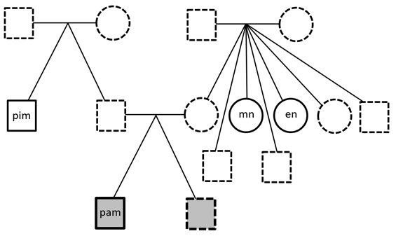

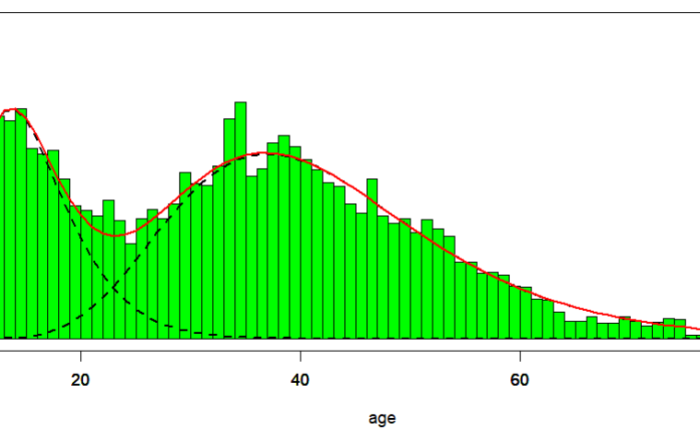


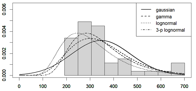
 is the Pearson correlation coefficient calculated for SBP and DBP;
  is the coefficient for CI and mean arterial pressure (MAP). MAP was calculated as DBP + (SBP – DBP)/3.
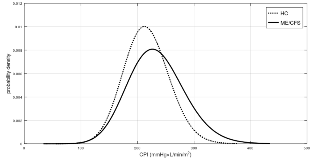

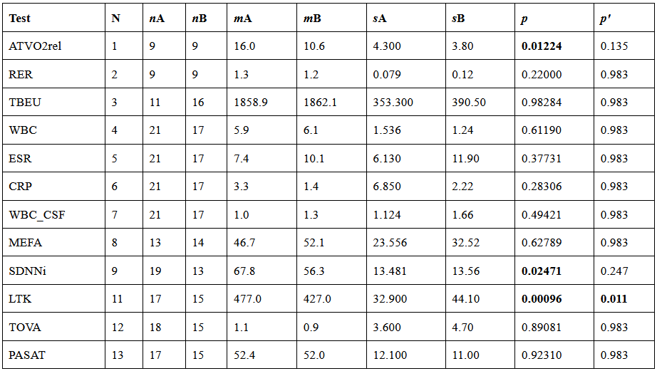
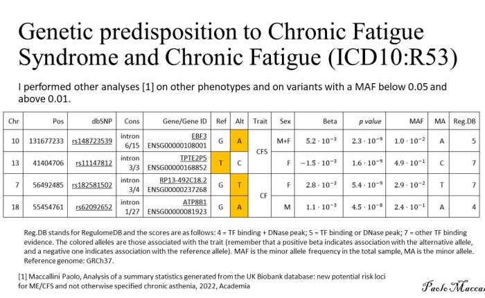


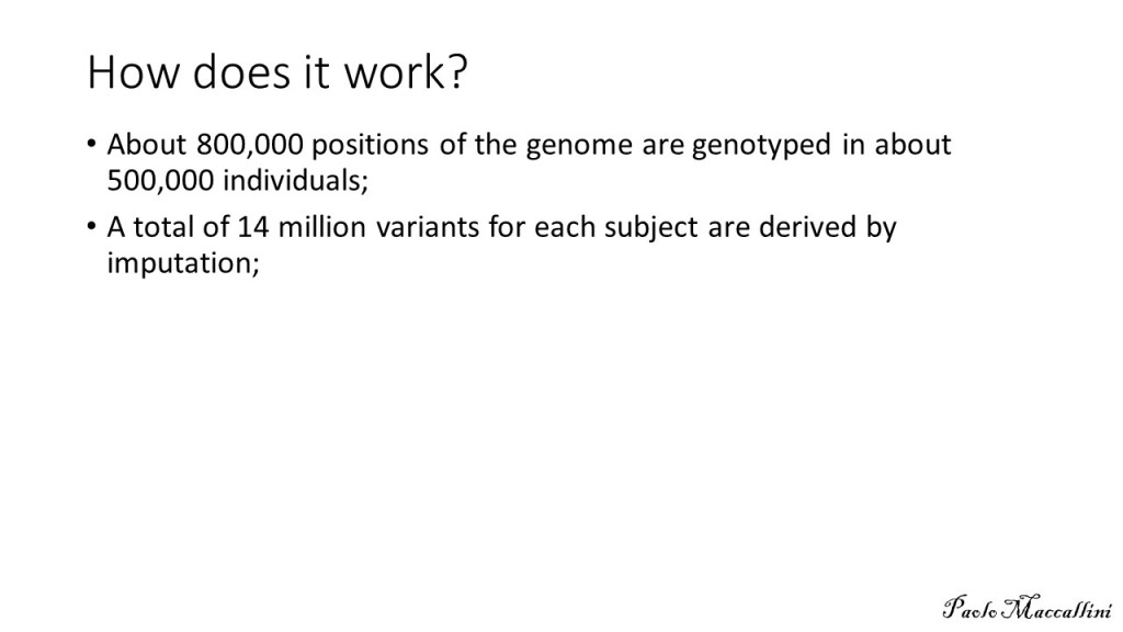


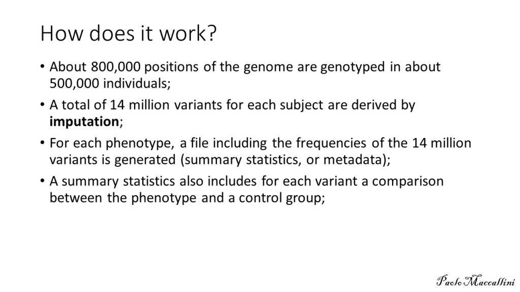


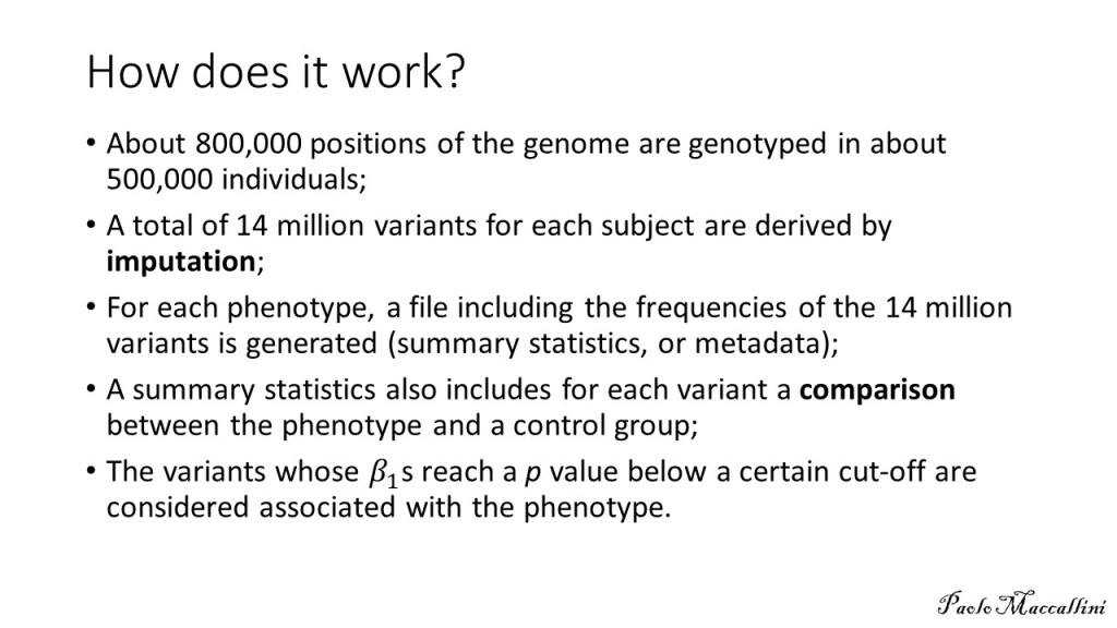
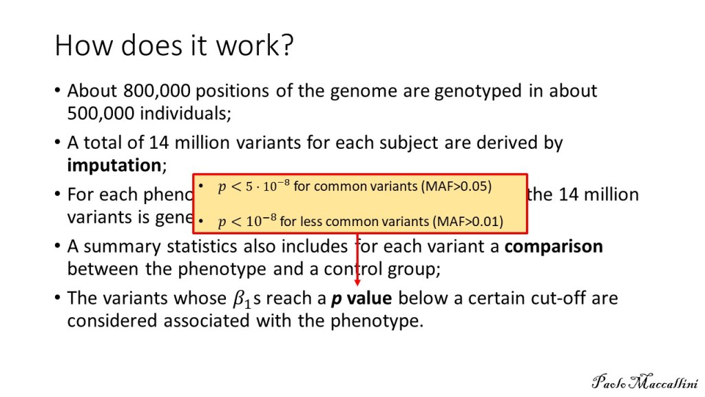


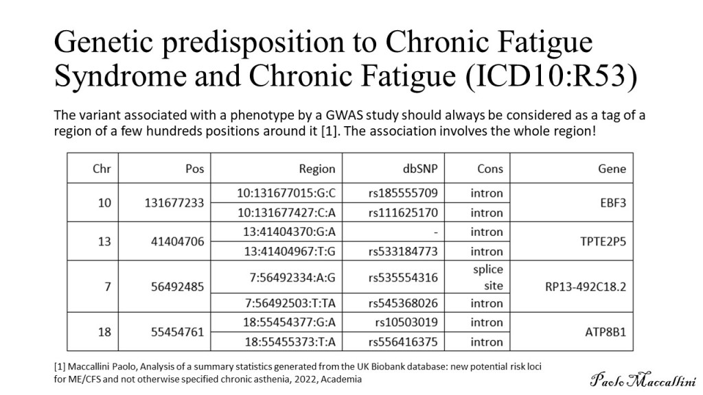


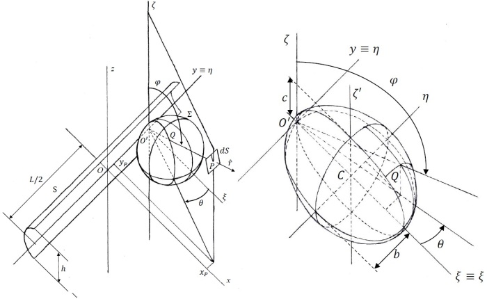
 . While the absence of correlation can be used to rule out causation, the presence of correlation does not mean automatically causation. Moreover, since air density and dry air density are strongly inversely correlated with air temperature, the correlations with air density might be driven by the correlation with air temperature (and vice-versa). In order to further investigate the nature of these correlations, I planned a second study, this time performed inside a chamber where I could manipulate the temperature of the air, the content of water in the air, and the amount of infrared radiation I was hit by. I called this chamber “Summer Simulator” because I used several devices to obtain, during the months from December to May, the conditions that we usually have in Rome during summer. I lived inside the simulator while I collected a functionality score, three times per day, and while I measured (every 10 minutes) the temperature of the air, relative humidity, and atmospheric pressure. The data for the months from January to April were used to study how my symptoms correlated with the environmental parameters I could directly measure and those that I could mathematically derive.

 . The temperature was controlled by a heat pump (Electrolux EXP26U558HW) that collects air from inside the room, divides it into two fluxes, transfers heat from one to the other (by cycles of compression-evaporation of refrigerant R290), and releases the warmer flux inside and the other one outside the window. The humidity was controlled by two/three ultrasonic mist humidifiers that release mist which is then turned into vapor in a fraction that depends on the temperature of the air (Figure 2).


 ).
).  is given by
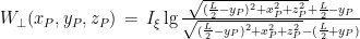
![I_\xi\,=\,\frac{e\Pi(1-4b^2)\sqrt{1-4c^2}}{8\pi hLbc[F(\arctan\sqrt{\frac{1-4c^2}{4c^2}},\sqrt{\frac{1-4b^2}{1-4c^2}})-E(\arctan\sqrt{\frac{1-4c^2}{4c^2}},\sqrt{\frac{1-4b^2}{1-4c^2}})]}](https://s0.wp.com/latex.php?latex=I_%5Cxi%5C%2C%3D%5C%2C%5Cfrac%7Be%5CPi%281-4b%5E2%29%5Csqrt%7B1-4c%5E2%7D%7D%7B8%5Cpi+hLbc%5BF%28%5Carctan%5Csqrt%7B%5Cfrac%7B1-4c%5E2%7D%7B4c%5E2%7D%7D%2C%5Csqrt%7B%5Cfrac%7B1-4b%5E2%7D%7B1-4c%5E2%7D%7D%29-E%28%5Carctan%5Csqrt%7B%5Cfrac%7B1-4c%5E2%7D%7B4c%5E2%7D%7D%2C%5Csqrt%7B%5Cfrac%7B1-4b%5E2%7D%7B1-4c%5E2%7D%7D%29%5D%7D&bg=ffffff&fg=000000&s=0&c=20201002)
 is the power absorbed by the device (about 800 W, according to the measurements performed by a power meter) and where F and E are the elliptic functions of the first and second kind, respectively (
 which is reached for b = 0.49, c = 0.36 (assuming c < b < 0.5).
 from O, is reported in figure 6, where it can be seen that the maximum of
  is reached for
 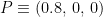 and its value is about 376
  .
. 
 , for
, for 
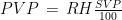
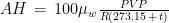
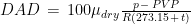

 is the molecular weight of water,
  is the molecular weight of dry air,
 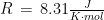 is the constant of gasses, and where we express temperature in °C and pressure in hPa. These formulae are taken from chapter 4 of the Guide to Instruments and Methods of Observation by the World Meteorological Organization (
 ; see figure 7.


 on the vertical plane by the left side of my bed, according to a mathematical model of the lamp (figure 6). This radiation was then partially reflected by the surfaces covered in mylar of my infrared chamber, so that it hit my body from other directions too, even though I have not built a model for the whole infrared chamber, yet.
 , where T is the temperature of the air at the level of the surface, expressed in Kelvin. But it should be noted that while 99% of the power emitted by the Earth as infrared radiation has a wavelength above
  , my infrared heater emits in the range
  . So, my artificial source of radiation does not simulate the radiation from the Earth, if we consider the wavelength (while it does from the point of view of the total power, as we will see in a following study, already concluded). But it could be considered that the radiation from the lamp did end up hitting the walls of my room, which in turn released their thermic energy as long wave infrared radiation. It is conceivable then that both in the Summer Simulator and in real summer, my improvements might be driven by far infrared radiation. Another possibility is that the improvement was due to the infrared radiation emitted by my body (long wave infrared radiation) and reflected back to me by the mylar coating of the infrared chamber.
 (PM2.5). The correlation between symptoms and air density and dry air density might be driven by the correlation with temperature because density is strongly inversely correlated with the temperature of the air.
  ) was converted from AQI (air quality index) to
  by solving the following equation with respect to C:
 and
and  are the ones collected in Table 1 and taken from (
 and then we solve Eq. 1 with respect to C to get the corresponding value of PM 2.5 in (
 is the partial pressure of water vapor in the air and
  is the saturation vapor pressure with respect to water (the vapor pressure in the air in equilibrium with the surface of the water). We then have
 , while
  is the temperature in °C and
  is the temperature in
  , with
  . Absolute humidity is simply given by
 is the mass of vapor and
  is the total volume occupied by the mixture (
 . Then, by substituting
  and
and  , we have
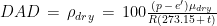
 . These calculations are reviewed in more detail in (
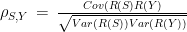


 )
)


 ) in the frequency of the alternative allele of variant
  ) with variant
  . I performed a similar analysis on chronic asthenia not otherwise specified (ICD10: R53) and I found an association between male patients and variant
  (read
(read  when testing the null hypothesis: the alleles are in HWE. I filtered out variants with expected minor allele count below 25, in cases.


 . Since the alternative variant is less frequent in patients than in controls, the prediction is that we have a reduced expression of