Spot Finder, a regression analysis

Abstract

My ME/CFS regularly improves during the summer. In a previous study, I found that the improvement correlates with air temperature but not with other environmental parameters. In a simulation of summerish conditions performed in a room, during cold months, by artificially increasing air temperature, infrared radiation, and air humidity, the correlation between my symptoms and air temperature tended to be negative. Here I report on a further study where I consider again environmental parameters from a few locations in the temperate and subtropical regions of both hemispheres and I search for the best regression model between them and my status (n=20). The best regression model, among the ones tested, is $Y=\beta_0+\beta_1 t +\beta_2 T^4$ where Y is my status (the higher the value, the less the symptoms), t is air temperature (°C) and T is absolute air temperature (K). This regression model approximates the flux of thermic energy between my body and the environment, when indoors, but with two different signs for the coefficients of t and of $T^4$ . I have used then the best regression model to predict the score over the year in several cities. These predictions can be used to find the optimal spot to live in, as a function of the month of the year.

Introduction

Figure 1. The duplets City-Month are reported in the euclidean space Cl, R, T. The points City-Months that have already been classified based on the score I registered for them, are colored green (score of 6), red (score of 4), yellow with a black contour line (score of 5), and yellow with a green contour line (score of 5.5). Black dots are doublets City-Month without a classification. CO = Corrientes, Argentina; AS = Asunción, Paraguay; SM = Santa Maria, Cape Verde. F = February; Ma = March, and so on.

Methods and Results

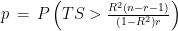
I have considered a set of 20 points defined by the two coordinates City and Month. To each of them, I have assigned a score, from 4 to 6, based on the degree of severity (the lower the score, the worse the disease) of my symptoms in that particular city, for that specific month. For each point City-Month I have collected the monthly mean air temperature (T), mean cloudiness (Cl), and mean solar radiation (R) (Figure 1). I have considered several models of regression between the score (response variable) and the three explanatory variables T, Cl, and R (Table 1). For each regression model, I have calculated the p values of the estimates of the coefficients, and I have also calculated the p value of the F test, given by

(1) $\,\,\,p\,=\,P\left(TS>\frac{R^2 \left(n-r-1\right)}{\left(1-R^2\right)r}\right)$

where TS follows an F law of parameters r and n-r-1, with r the number of explanatory variables and n the number of data points. All the calculations and the plots of this article (except for Figure 3) have been performed by two custom scripts (reported at the end), one in Octave, and one in R. For the script in Octave I wrote a subroutine for the F-test. The R script also calculates Spearman’s, and Pearson’s correlation coefficients between the variables, including their p values and the corrections for temperature (Table 2).

Table 1. For each regression model, I have indicated the values of the estimates of the coefficients (with their degree of significance), and the p value of the F test. The meaning of the asterisks is * p < 0.05; ** p<0.001; *** p = 0. T = mean daily absolute temperature; t = meant daily temperature in Celsius, R = mean daily solar radiation; Cl = fraction of the day mainly cloudy.

I have used then the best regression model to predict the score along the year in several cities in the temperate and subtropical regions of both hemispheres (Figure 2). The diagrams have been interpolated by using cubic splines, to make them more smooth. These predictions can be used to find the best spot to live in, as a function of the month of the year.

Figure 2. Prediction for the score by the regression model $Y=\beta_0+\beta_1 T^4$ . RM = Rome; AR = Arona, Tenerife, Spain; RO = Rosario, Argentina; BA = Buenos Aires, Argentina; AS = Asunción, Paraguay; CO = Corrientes, Argentina; SM = Santa Maria, Cape Verde.

Table 2. Correlation coefficients (Spearman and Person) between the variables. Corrected Pearson correlations were also computed, when possible. T = mean daily absolute temperature; t = meant daily temperature in Celsius, R = mean daily solar radiation; Cl = fraction of the day mainly cloudy.

I also used the 198 data points from my previous study (Maccallini P. 2022) to test models 7 and 6 of regression. I considered the mean data on three days for all the variables (Table 3). In this case, model 6 performs better. We still have a good level of significance in the F test, and we still have a negative coefficient for t in model 7. If we use this model to make previsions on the score as a function of the month in various cities, we get Figure 3. Consider that this regression model is based on a scoring system that is slightly lower if compared with the one used for the previous analysis.

Table 3. For each regression model, I have indicated the values of the estimates of the coefficients (with their degree of significance), and the p value of the F test. The meaning of the asterisks is: . p<01, * p < 0.05; ** p<0.001; *** p = 0. T = mean daily absolute temperature; t = meant daily temperature in Celsius, R = mean daily solar radiation; Cl = fraction of the day mainly cloudy.

Figure 2. Prediction for the score by the regression model 6 of Table 3. RM = Rome; AR = Arona, Tenerife, Spain; RO = Rosario, Argentina; BA = Buenos Aires, Argentina. AS = Asunción, Paraguay; CO = Corrientes, Argentina; SM = Santa Maria, Cape Verde.

Discussion

The best regression model is $Y=\beta_0+\beta_1 t +\beta_2 T^4$ , followed by the model $\beta_0+\beta_1 T^4$ , and model $Y=\beta_0+\beta_1 R +\beta_2 t + \beta_3 T^4$ . These three models have a physical meaning; namely, they express the flux of thermic energy between my body and the environment. The human body must balance the energy exchanged with the environment to maintain thermic homeostasis. The power P exchanged with the environment can be written as

(2) $\,\,\,P\,=\,R+CV+CD+E$

where R is the power exchange in the form of radiant energy, C is the exchange by conduction, CV is the exchange by convection, and E is the dispersion of power by evaporation. This is a simplification of complex phenomena that should also take into account the exchange of thermic power associated with the passage of atmospheric gas through the respiratory system. The power R can be further specified in the form $R\,=\,K_1 R_{sun} + K_2(T_me^4-T_env^4)$ where $K_1 R_{sun}$ is the power absorbed from the Sun, and the other addend is the radiant power exchanged with the environment, whit $K_2$ a constant that expresses radiant and geometrical properties of both my body and of the environment. While $R_{sun}$ is radiant power in the form of short wave radiation (wavelength below 3 $\mu$ ), the other addend represents radiant power exchanged by bodies at low temperatures with a wavelength above 3 $\mu$ (according to the Stephan-Boltzman law) (R). But what temperature is $T_{env}$ ? One first approximation might be the absolute temperature of the air, because in warm months, with the windows open, the objects surrounding us tend to acquire a superficial temperature similar to that of the air. To show that point, I analyzed the power emitted by the soil in Rome, during the year 2020, and the temperature of the air (data from ARPALAZIO). If we indicate J the daily mean power emitted per surface unit by the soil in the hemispace, the Stefan-Boltzmann law states that

(3) $\,\,\,J\,=\,a\chi T_s^4$

where a is a constant below 1 dependent on the material of the surface of the soil, $\chi\,=\,5.6696\cdot10^{-8}\frac{W}{m^2 K^4}$ is the Stefan-Boltzmann constant, and $T_s$ is the absolute temperature of the soil. If the assertion that the temperature of the soil is about the same as the temperature of the air was correct, the regression for the following linear model should have a very low p value of the F test:

(4) $\,\,\,J\,=\,B_0 + B_1(273.15 + t_a)^4$

And this is in fact the case, we have the regression in Figure 3, with a p value of the F test below $2.2\cdot 10^{-16}$ . For further details on these calculations, see (Maccallini P, 2022).

Figure 3. Linear regression between the mean daily irradiance from the Earth and the fourth power of the absolute temperature of the air (daily mean value). Data from ARPA, Rome, 2020. The analysis is described in detail in (Maccallini P, 2022).

As for the exchange of power by conduction and convection, in both cases, they are expressed by a constant multiplied by the difference in temperature between my skin and the air. That said, we can write again eq. 1 as follows:

(5) $\,\,\,P\,=\,K_1 R_{sun}+K_2 (T_{skin}^4-T_{air}^4)+K_3 (t_{skin} - t_{air})$

were we have removed the term linked to evaporation. In other words, the power exchanged by my body with the environment could be expressed, in first approximation, by the equation

(6) $\,\,\,P\,=\,B_0+B_1 R_{sun}+B_2 t_{air} + B_3 T_{air}^4$

This is model 5 of Table 1. If we consider the case of a subject who rarely leaves home, we can get rid of $R_{sun}$ and we get model 7, the best model of regression. In a previous article, I showed that the best correlation between my status and several environmental parameters was with air temperature (R), and yet in an experiment where I simulated summer in a room with the use of a heat pump, an infrared lamp, and an air moisturizer, there was no correlation between my status and air temperature (R) (in fact the correlation had a tendency to be negative). From the perspective of this new study, I would explain the previous results as follows: in the first study performed during worm months using environmental parameters we caught the Spearman’s correlation between my status and air temperature which was a reflection of the correlation between my status and the longwave infrared radiation from the environment (proportional to the fourth power of the absolute temperature of the air); in the second study, performed during cold months within a room with artificially heated air, there was no correlation between air temperature and the infrared emission of the environment (which came from a lamp), so we found a correlation that tended to be negative perhaps because when I was feeling worse I raised the temperature of the air. It should be noted though that in models 7 and 5 the coefficient of t is negative, therefore it seems that while the longwave infrared radiation plays a positive role, the temperature of the air does not.

Conclusion

The three best regression models suggest that my improvement is linked to the thermal energy balance of the body: the lower the dispersion of radiant thermic energy, the better I feel. But at the same time, the temperature of the air has a detrimental effect. But other interpretations might be possible: there might be an effect of thermal radiation on my biology that is not linked to thermic homeostasis but instead to some other biological targets. Moreover, there might be other models of regression that I have not considered, that perform better than the ones mentioned.

Scripts

The first script is written in Octave. It calculates the regressions and their F tests (by using a custom subroutine) and it plots Figure 1 and Figure 2. It also writes the data in csv format for the second script (in R), which performs the same statistical analyses and also calculates the p values associated with each coefficient estimate.

% file name = Spot_finder_2
% date of creation = 29/01/2023
%
close all
clear all
#
pkg load statistics % we need this package for the F law
spline = 1 % it is one if we want a cubic spline interpolation for the last plot
#
#-------------------------------------------------------------------------------
# Data
#-------------------------------------------------------------------------------
#
months = ["Je"; "F"; "Mr"; "Ap"; "Ma"; "Jn"; "Jl"; "Au"; "S"; "O"; "N"; "D"];
%
% data of Rome (RM), Italy
%
k=1;
Spot(1,:,k) = [2,3,4.3,5.6,6.8,7.5,7.5,6.5,4.9,3.4,2.2,1.8]; % Mean daily incident solar radiation (kWh/m^2)
Spot(2,:,k) = [47,44,44,43,39,25,13,18,32,43,47,46]; % Fraction of the day mainly cloudy (%)
Spot(3,:,k) = [7,8,11,13,18,22,25,25,21,17,12,8]; % Mean air temperature (°C)
Spot(4,:,k) = [3,3,6,8,12,16,18,18,15,12,7,4]; % Min air temperature (°C)
Spot(5,:,k) = [12,13,16,19,23,27,31,31,27,22,17,13]; % Max air temperature (°C)
%
% data of Arona (AR), Tenerife, Spain
%
k=2;
Spot(1,:,k) = [3.9,4.9,6.1,7.2,7.8,8.2,8.0,7.4,6.3,5.1,4.0,3.5]; % Mean daily incident solar radiation (kWh/m^2)
Spot(2,:,k) = [32,28,26,24,21,9,2,6,21,34,38,36]; % Fraction of the day mainly cloudy (%)
Spot(3,:,k) = [19,19,19,20,21,22,24,25,25,24,22,20]; % Mean air temperature (°C)
Spot(4,:,k) = [16,16,16,17,18,20,21,22,22,21,19,17]; % Min air temperature (°C)
Spot(5,:,k) = [22,22,23,23,24,26,28,28,28,27,25,23]; % Max air temperature (°C)
%
% data of Rosario (RO), Santa Fe, Argentina
%
k=3;
Spot(1,:,k) = [7.6,6.7,5.6,4.3,3.2,2.7,3.0,3.9,5.1,6.3,7.3,7.7]; % Mean daily incident solar radiation (kWh/m^2)
Spot(2,:,k) = [28,28,28,34,45,47,44,40,36,32,30,28]; % Fraction of the day mainly cloudy (%)
Spot(3,:,k) = [25,23,22,18,14,11,10,12,15,18,21,24]; % Mean air temperature (°C)
Spot(4,:,k) = [19,18,17,13,10,7,6,7,9,13,16,18]; % Min air temperature (°C)
Spot(5,:,k) = [30,29,27,23,19,16,16,18,21,24,27,29]; % Max air temperature (°C)
%
% data of Buenos Aires (BA), Argentina
%
k=4;
Spot(1,:,k) = [7.6,6.7,5.5,4.1,3.0,2.5,2.7,3.6,4.8,6.2,7.3,7.8]; % Mean daily incident solar radiation (kWh/m^2)
Spot(2,:,k) = [29,31,31,38,48,50,48,45,41,37,33,30]; % Fraction of the day mainly cloudy (%)
Spot(3,:,k) = [24,23,22,18,15,12,11,13,14,17,20,23]; % Mean air temperature (°C)
Spot(4,:,k) = [21,20,19,15,12,9,9,10,11,14,17,19]; % Min air temperature (°C)
Spot(5,:,k) = [28,27,25,21,18,15,14,16,18,21,24,27]; % Max air temperature (°C)
%
% data of Asuncion (AS), Paraguay
%
k=5;
Spot(1,:,k) = [7.0,6.6,6.0,5.0,4.1,3.5,3.8,4.5,5.3,6.1,6.9,7.1]; % Mean daily incident solar radiation (kWh/m^2)
Spot(2,:,k) = [45,42,33,31,32,37,35,32,32,38,38,42]; % Fraction of the day mainly cloudy (%)
Spot(3,:,k) = [28,27,26,23,20,18,18,20,21,24,25,27]; % Mean air temperature (°C)
Spot(4,:,k) = [23,23,21,19,16,14,14,15,16,19,21,22]; % Min air temperature (°C)
Spot(5,:,k) = [33,32,31,28,25,23,23,25,27,29,31,32]; % Max air temperature (°C)
%
% data of Corrientes (CO), Argentina
%
k=6;
Spot(1,:,k) = [7.2,6.7,5.9,4.8,3.9,3.4,3.6,4.3,5.3,6.2,7.0,7.3]; % Mean daily incident solar radiation (kWh/m^2)
Spot(2,:,k) = [39,35,30,30,33,37,35,33,32,34,34,36,]; % Fraction of the day mainly cloudy (%)
Spot(3,:,k) = [27,26,25,22,18,16,15,17,19,22,24,26]; % Mean air temperature (°C)
Spot(4,:,k) = [22,22,20,17,14,12,11,12,14,17,19,21]; % Min air temperature (°C)
Spot(5,:,k) = [33,32,30,26,23,21,21,23,25,27,29,31]; % Max air temperature (°C)
%
% data of SantaMaria (SM), Capo Verde
%
k=7;
Spot(1,:,k) = [5.0,5.9,6.8,7.3,7.3,7.2,6.7,6.2,5.8,5.6,5.0,4.6]; % Mean daily incident solar radiation (kWh/m^2)
Spot(2,:,k) = [42,35,34,33,25,19,36,53,56,48,54,49]; % Fraction of the day mainly cloudy (%)
Spot(3,:,k) = [22,22,22,22,23,24,25,27,27,27,25,23]; % Mean air temperature (°C)
Spot(4,:,k) = [20,19,20,20,21,22,23,25,25,24,23,21]; % Min air temperature (°C)
Spot(5,:,k) = [25,25,25,26,26,27,28,30,30,30,28,26]; % Max air temperature (°C)
%
names = {"RM","AR","RO","BA","AS","CO","SM"};
types = {"-k","--k",":k","-r","--r",":r","-b","--b","-.b",}
%
for i=1:5
  max_measure(i) = max([Spot(i,:,1),Spot(i,:,2),Spot(i,:,3),Spot(i,:,4),Spot(i,:,5),Spot(i,:,6),Spot(i,:,7)])
endfor
%
%-------------------------------------------------------------------------------
% Subroutine for F-test
%-------------------------------------------------------------------------------
%
function [pval,R2,TS] = F_test (M,b,beta)
  r = length(M(1,:))-1; % number of explanatory variables
  n = length(M(:,1)) % number of data points
  R = b-M*beta; % residues
  SSR = 0;
  Sbb = 0;
  for i=1:n
    SSR = SSR + R(i)^2; % sum of squared residues
    Sbb = Sbb + b(i)^2;
  endfor
  Sbb = Sbb - n*(mean(b))^2;
  R2 = (Sbb - SSR)/Sbb; % R squared
  TS = R2*(n-r-1)/(r*(1-R2)); % test statistics
  pval = 1 - fcdf(TS,r,n-r-1); % F-test
endfunction
%
%-------------------------------------------------------------------------------
% Subroutine plot_score
%-------------------------------------------------------------------------------
%
function Plot_score (score, h, model, names, types, spline)
    figure(5) % Plotting of the Scoring for the query spots
    %
    for k=1:length(names)
      if (spline==1)
        yi = interp1([1:1:12],score(:,k),[1:0.25:12],"spline")
        plot([1:0.25:12],yi,char(types{k}),"linewidth",1.5)
        hold on
      else
        plot([1:1:12],score(:,k),char(types{k}),"linewidth",1.5)
        hold on
      endif
    endfor
    plot([1,12],[5,5],"--g","linewidth",1.5)
    title(model{h})
    legend(char(names{1:length(names)}),"location","southwest",'fontsize',15)
    xlabel("Month",'fontsize',15);
    ylabel("Score",'fontsize',15);
    grid on
    grid minor on
endfunction
%
%-------------------------------------------------------------------------------
figure 1 % mean temp, irradiation, cloudiness with storing of data for regressions
%-------------------------------------------------------------------------------
%
% plotting Rome
%
k=1;
n=1;
for i=1:12
  if (and(i>=6,i<9))
    plot3(Spot(1,i,k),Spot(2,i,k),Spot(3,i,k),'o','markersize',6,'markerfacecolor','g','markeredgecolor','k')
    b(n)=6;
    M(n,1:4)=[1,Spot(1,i,k),Spot(2,i,k),Spot(3,i,k)];
    n=n+1
  endif
  if (or(i<6,i>9))
    plot3(Spot(1,i,k),Spot(2,i,k),Spot(3,i,k),'o','markersize',6,'markerfacecolor','r','markeredgecolor','k')
  endif
  if (or(and(i>3,i<5),i>9))
    b(n)=4;
    M(n,1:4)=[1,Spot(1,i,k),Spot(2,i,k),Spot(3,i,k)];
    n=n+1
  endif
  if (i==5)
    b(n)=5;
    M(n,1:4)=[1,Spot(1,i,k),Spot(2,i,k),Spot(3,i,k)];
    n=n+1
  endif
  if (i==9)
    plot3(Spot(1,i,k),Spot(2,i,k),Spot(3,i,k),'o','markersize',6,'markerfacecolor','y','markeredgecolor','g')
    b(n)=5.7;
    M(n,1:4)=[1,Spot(1,i,k),Spot(2,i,k),Spot(3,i,k)];
    n=n+1
  endif
  hold on
endfor
%
% plotting Arona
%
k=2;
for i=1:12
  if (i==5)
    plot3(Spot(1,i,k),Spot(2,i,k),Spot(3,i,k),'o','markersize',6,'markerfacecolor','g','markeredgecolor','k')
    b(n)=6
    M(n,1:4)=[1,Spot(1,i,k),Spot(2,i,k),Spot(3,i,k)];
    n=n+1
  endif
  if (and(i>=1,i<5))
    plot3(Spot(1,i,k),Spot(2,i,k),Spot(3,i,k),'o','markersize',6,'markerfacecolor','r','markeredgecolor','k')
    b(n)=4
    M(n,1:4)=[1,Spot(1,i,k),Spot(2,i,k),Spot(3,i,k)];
    n=n+1
  endif
    hold on
endfor
%
% plotting Rosario
%
k=3;
for i=1:12
  if (and(i>=1,i<3))
    plot3(Spot(1,i,k),Spot(2,i,k),Spot(3,i,k),'o','markersize',6,'markerfacecolor','g','markeredgecolor','k')
    b(n)=6
    M(n,1:4)=[1,Spot(1,i,k),Spot(2,i,k),Spot(3,i,k)];
    n=n+1
  endif
  if (i==3)
    plot3(Spot(1,i,k),Spot(2,i,k),Spot(3,i,k),'o','markersize',6,'markerfacecolor','y','markeredgecolor','k')
    b(n)=5.5
    M(n,1:4)=[1,Spot(1,i,k),Spot(2,i,k),Spot(3,i,k)];
    n=n+1
  endif
  hold on
endfor
%
% plotting CABA
%
k=4;
for i=1:12
  if (or(i==12,i==1,i==2))
    plot3(Spot(1,i,k),Spot(2,i,k),Spot(3,i,k),'o','markersize',6,'markerfacecolor','g','markeredgecolor','k')
    b(n)=6
    M(n,1:4)=[1,Spot(1,i,k),Spot(2,i,k),Spot(3,i,k)];
    n=n+1
  endif
  if (i<12)
    hold on
  endif
endfor
%
% plotting query spots
%
% Asuncion
%
k=5;
for i=2:4
  plot3(Spot(1,i,k),Spot(2,i,k),Spot(3,i,k),'o','markersize',6,'markerfacecolor','k','markeredgecolor','k')
  text(Spot(1,i,k),Spot(2,i,k),Spot(3,i,k)+0.5, strcat(char(names{k}),", ",months(i,:)),'fontsize',15)
endfor
%
% Corrientes
%
k=6;
for i=2:4
  plot3(Spot(1,i,k),Spot(2,i,k),Spot(3,i,k),'o','markersize',6,'markerfacecolor','k','markeredgecolor','k')
  text(Spot(1,i,k),Spot(2,i,k),Spot(3,i,k)+0.5, strcat(char(names{k}),", ",months(i,:)),'fontsize',15)
endfor
%
% Santa Maria
%
k=7;
for i=2:5
  plot3(Spot(1,i,k),Spot(2,i,k),Spot(3,i,k),'o','markersize',6,'markerfacecolor','k','markeredgecolor','k')
  text(Spot(1,i,k),Spot(2,i,k),Spot(3,i,k)+0.5, strcat(char(names{k}),", ",months(i,:)),'fontsize',15)
endfor
%
grid on
grid minor on
xlabel("Mean daily incident solar radiation (kWh/m^{2})",'fontsize',15);
ylabel("Fraction of the day mainly cloudy (%)",'fontsize',15);
zlabel("Mean air temperature (°C)",'fontsize',15);
axis ('square')
axis([4,max_measure(1),0,max_measure(2),15,max_measure(3)])
%
%-------------------------------------------------------------------------------
% Regressions
%-------------------------------------------------------------------------------
%
n=n-1; % number of measures
%
b = transpose(b)
x = cell() % it contains the coefficients of the models
model = cell() % it contains the description of the models
matrix = cell() % it contains the matrix of the regression
k = 0;
%
for i=1:n
  A(i,1:3)=[1,M(i,2),M(i,4)]
endfor
k = k+1;
[x{k}, std, mse, S] = lscov (A, b)
[pval(k), R2(k), TS(k)] = F_test (A, b, x{k})
model{k} = "socre = b0 + b1*Rad + b2*t"
matrix{k} = A;
clear A
%
for i=1:n
  A(i,1:3)=[1,M(i,3),M(i,4)]
endfor
k = k+1;
[x{k}, std, mse, S] = lscov (A, b)
[pval(k), R2(k), TS(k)] = F_test (A, b, x{k})
model{k} = "socre = b0 + b1*Cl + b2*t"
matrix{k} = A;
clear A
%
for i=1:n
  A(i,1:4)=[1,M(i,2),M(i,3),M(i,4)]
endfor
k = k+1;
[x{k}, std, mse, S] = lscov (A, b)
[pval(k), R2(k), TS(k)] = F_test (A, b, x{k})
model{k} = "socre = b0 + b1*Rad + b1*Cl + b2*t"
matrix{k} = A;
clear A
%
for i=1:n
  A(i,1:3)=[1,M(i,2),(273.15+M(i,4))^4]
endfor
k = k+1;
[x{k}, std, mse, S] = lscov (A, b)
[pval(k), R2(k), TS(k)] = F_test (A, b, x{k})
model{k} = "socre = b0 + b1*Rad + b2*T^{4}"
matrix{k} = A;
clear A
%
for i=1:n
  A(i,1:4)=[1,M(i,2),M(i,4),(273.15+M(i,4))^4]
endfor
k = k+1;
[x{k}, std, mse, S] = lscov (A, b)
[pval(k), R2(k), TS(k)] = F_test (A, b, x{k})
model{k} = "socre = b0 + b1*Rad + b2*t + b3*T^{4}"
matrix{k} = A;
clear A
%
for i=1:n
  A(i,1:2)=[1,(273.15+M(i,4))^4]
endfor
k = k+1;
[x{k}, std, mse, S] = lscov (A, b)
[pval(k), R2(k), TS(k)] = F_test (A, b, x{k})
model{k} = "socre = b0 + b1*T^{4}"
matrix{k} = A;
clear A
%
for i=1:n
  A(i,1:3)=[1,M(i,4),(273.15+M(i,4))^4]
endfor
k = k+1;
[x{k}, std, mse, S] = lscov (A, b)
[pval(k), R2(k), TS(k)] = F_test (A, b, x{k})
model{k} = "socre = b0 + b1*t + b2*T^{4}"
matrix{k} = A;
clear A
%
%-------------------------------------------------------------------------------
% Selection of the best model
%-------------------------------------------------------------------------------
%
for i=1:length(pval)
  if (pval(i)==min(pval))
    best=i;
  endif
endfor
%
%-------------------------------------------------------------------------------
% Region of the plane Rad-Temp with high score according to the regression
% model
%-------------------------------------------------------------------------------
%
R(1)= 4;
R(2)= max_measure(1);
Temp_R(1) = ( 5.5 - x{1}(1) - x{1}(2)*R(1) )/x{1}(3);
Temp_R(2) = ( 5.5 - x{1}(1) - x{1}(2)*R(2) )/x{1}(3);
%
%-------------------------------------------------------------------------------
% Region of the plane Cloudiness-Temp with high score according to the regression
% model
%-------------------------------------------------------------------------------
%
Cl(1)= 0;
Cl(2)= max_measure(2);
Temp_Cl(1) = ( 5.5 - x{2}(1) - x{2}(2)*Cl(1) )/x{2}(3);
Temp_Cl(2) = ( 5.5 - x{2}(1) - x{2}(2)*Cl(2) )/x{2}(3);
%
%-------------------------------------------------------------------------------
figure 2 % mean temp and irradiation
%-------------------------------------------------------------------------------
%
% plotting Rome
%
k=1;
for i=1:12
  if (and(i>=6,i<9))
    plot(Spot(1,i,k),Spot(3,i,k),'o','markersize',6,'markerfacecolor','g','markeredgecolor','k')
  endif
  if (or(i<6,i>9))
    plot(Spot(1,i,k),Spot(3,i,k),'o','markersize',6,'markerfacecolor','r','markeredgecolor','k')
  endif
  if (i==9)
    plot(Spot(1,i,k),Spot(3,i,k),'o','markersize',6,'markerfacecolor','y','markeredgecolor','g')
  endif
  hold on
endfor
%
% plotting Arona
%
k=2;
for i=1:12
  if (i==5)
    plot(Spot(1,i,k),Spot(3,i,k),'o','markersize',6,'markerfacecolor','g','markeredgecolor','k')
  endif
  if (and(i>=1,i<5))
    plot(Spot(1,i,k),Spot(3,i,k),'o','markersize',6,'markerfacecolor','r','markeredgecolor','k')
  endif
    hold on
endfor
%
% plotting Rosario
%
k=3;
for i=1:12
  if (and(i>=1,i<3))
    plot(Spot(1,i,k),Spot(3,i,k),'o','markersize',6,'markerfacecolor','g','markeredgecolor','k')
  endif
  if (i==3)
    plot(Spot(1,i,k),Spot(3,i,k),'o','markersize',6,'markerfacecolor','y','markeredgecolor','k')
  endif
  hold on
endfor
%
% plotting CABA
%
k=4;
for i=1:12
  if (or(i==12,i==1,i==2))
    plot(Spot(1,i,k),Spot(3,i,k),'o','markersize',6,'markerfacecolor','g','markeredgecolor','k')
  endif
  if (i<12)
    hold on
  endif
endfor
%
% plotting query spots
%
% Asuncion
%
k=5;
for i=2:4
  plot(Spot(1,i,k),Spot(3,i,k),'o','markersize',6,'markerfacecolor','k','markeredgecolor','k')
  text(Spot(1,i,k),Spot(3,i,k)+0.5, strcat(char(names{k}),", ",months(i,:)),'fontsize',15)
endfor
%
% Corrientes
%
k=6;
for i=2:4
  plot(Spot(1,i,k),Spot(3,i,k),'o','markersize',6,'markerfacecolor','k','markeredgecolor','k')
  text(Spot(1,i,k),Spot(3,i,k)+0.5, strcat(char(names{k}),", ",months(i,:)),'fontsize',15)
endfor
%
% Santa Maria
%
k=7;
for i=3:5
  plot(Spot(1,i,k),Spot(3,i,k),'o','markersize',6,'markerfacecolor','k','markeredgecolor','k')
  text(Spot(1,i,k),Spot(3,i,k)+0.5, strcat(char(names{k}),", ",months(i,:)),'fontsize',15)
endfor
%
plot([R(1),R(2)],[Temp_R(1),Temp_R(2)],"--k","linewidth",1)
%
grid on
grid minor on
xlabel("Mean daily incident solar radiation (kWh/m^{2})",'fontsize',15);
ylabel("Mean air temperature (°C)",'fontsize',15);
axis([R(1),R(2),15,max_measure(3)])
%
%-------------------------------------------------------------------------------
figure 3 % mean temp and cloudiness
%-------------------------------------------------------------------------------
%
% plotting Rome
%
k=1;
for i=1:12
  if (and(i>=6,i<9))
    plot(Spot(2,i,k),Spot(3,i,k),'o','markersize',6,'markerfacecolor','g','markeredgecolor','k')
  endif
  if (or(i<6,i>9))
    plot(Spot(2,i,k),Spot(3,i,k),'o','markersize',6,'markerfacecolor','r','markeredgecolor','k')
  endif
  if (i==9)
    plot(Spot(2,i,k),Spot(3,i,k),'o','markersize',6,'markerfacecolor','y','markeredgecolor','g')
  endif
  hold on
endfor
%
% plotting Arona
%
k=2;
for i=1:12
  if (i==5)
    plot(Spot(2,i,k),Spot(3,i,k),'o','markersize',6,'markerfacecolor','g','markeredgecolor','k')
  endif
  if (and(i>=1,i<5))
    plot(Spot(2,i,k),Spot(3,i,k),'o','markersize',6,'markerfacecolor','r','markeredgecolor','k')
  endif
    hold on
endfor
%
% plotting Rosario
%
k=3;
for i=1:12
  if (and(i>=1,i<3))
    plot(Spot(2,i,k),Spot(3,i,k),'o','markersize',6,'markerfacecolor','g','markeredgecolor','k')
  endif
  if (i==3)
    plot(Spot(2,i,k),Spot(3,i,k),'o','markersize',6,'markerfacecolor','y','markeredgecolor','k')
  endif
  hold on
endfor
%
% plotting CABA
%
k=4;
for i=1:12
  if (or(i==12,i==1,i==2))
    plot(Spot(2,i,k),Spot(3,i,k),'o','markersize',6,'markerfacecolor','g','markeredgecolor','k')
  endif
  if (i<12)
    hold on
  endif
endfor
%
% plotting query spots
%
% Buenos Aires
%
i=2;
k=4;
plot(Spot(2,i,k),Spot(3,i,k),'o','markersize',6,'markerfacecolor','k','markeredgecolor','k')
text(Spot(2,i,k),Spot(3,i,k)-0.5, strcat(char(names{k}),", ",months(i,:)),'fontsize',15)
%
% Asuncion
%
k=5;
for i=2:4
  plot(Spot(2,i,k),Spot(3,i,k),'o','markersize',6,'markerfacecolor','k','markeredgecolor','k')
  text(Spot(2,i,k),Spot(3,i,k)+0.5, strcat(char(names{k}),", ",months(i,:)),'fontsize',15)
endfor
%
% Corrientes
%
k=6;
for i=2:4
  plot(Spot(2,i,k),Spot(3,i,k),'o','markersize',6,'markerfacecolor','k','markeredgecolor','k')
  text(Spot(2,i,k),Spot(3,i,k)-0.5, strcat(char(names{k}),", ",months(i,:)),'fontsize',15)
endfor
%
% Santa Maria
%
k=7;
for i=3:5
  plot(Spot(2,i,k),Spot(3,i,k),'o','markersize',6,'markerfacecolor','k','markeredgecolor','k')
  text(Spot(2,i,k),Spot(3,i,k)+0.5, strcat(char(names{k}),", ",months(i,:)),'fontsize',15)
endfor
%
plot([Cl(1),Cl(2)],[Temp_Cl(1),Temp_Cl(2)],"--k","linewidth",1)
%
grid on
grid minor on
xlabel("Fraction of the day mainly cloudy (%)",'fontsize',15);
ylabel("Mean air temperature (°C)",'fontsize',15);
axis([Cl(1),Cl(2),15,max_measure(3)])
%
%-------------------------------------------------------------------------------
% Plotting the scoring for each city according to the best model
%-------------------------------------------------------------------------------
%
switch best
  case 1
    %
    % Scoring for the query spots according to model h
    %
    h=1;
    for i=1:12
      for k=1:length(names)
        score(i,k) = x{h}(1)+x{h}(2)*Spot(1,i,k)+x{h}(3)*Spot(3,i,k);
      endfor
    endfor
    %
    figure(5) % Plotting of the Scoring for the query spots
    %
    for k=1:length(names)
      plot([1:1:12],score(:,k),char(types{k}),"linewidth",1.5)
      hold on
    endfor
    plot([1,12],[5,5],"--g","linewidth",1.5)
    title(model{h},'fontsize',15)
    legend(char(names{1:length(names)}),"location","southwest",'fontsize',15)
    xlabel("Month",'fontsize',15);
    ylabel("Score",'fontsize',15);
    grid on
    grid minor on
  case 2
    %
    % Scoring for the query spots according to model h 
    %
    h=2;
    for i=1:12
      for k=1:length(names)
        score(i,k) = x{h}(1)+x{h}(2)*Spot(2,i,k)+x{h}(3)*Spot(3,i,k);
      endfor
    endfor
    %
    figure(5) % Plotting of the Scoring for the query spots
    %
    for k=1:length(names)
      plot([1:1:12],score(:,k),char(types{k}),"linewidth",1.5)
      hold on
    endfor
    plot([1,12],[5,5],"--g","linewidth",1.5)
    title(model{h},'fontsize',15)
    legend(char(names{1:length(names)}),"location","southwest",'fontsize',15)
    xlabel("Month",'fontsize',15);
    ylabel("Score",'fontsize',15);
    grid on
    grid minor on
  case 3
    %
    % Scoring for the query spots according to model h
    %
    h=3;
    for i=1:12
      for k=1:length(names)
        score(i,k) = x{h}(1)+x{h}(2)*Spot(1,i,k)+x{h}(3)*Spot(2,i,k)+x{h}(4)*Spot(3,i,k);
      endfor
    endfor
    %
    figure(5) % Plotting of the Scoring for the query spots
    %
    for k=1:length(names)
      plot([1:1:12],score(:,k),char(types{k}),"linewidth",1.5)
      hold on
    endfor
    plot([1,12],[5,5],"--g","linewidth",1.5)
    title(model{h},'fontsize',15)
    legend(char(names{1:length(names)}),"location","southwest",'fontsize',15)
    xlabel("Month",'fontsize',15);
    ylabel("Score",'fontsize',15);
    grid on
    grid minor on
  case 4
    %
    % Scoring for the query spots according to model h
    %
    h=4;
    for i=1:12
      for k=1:length(names)
        score(i,k) = x{h}(1)+x{h}(2)*Spot(1,i,k)+x{h}(3)*(Spot(3,i,k)^4);
      endfor
    endfor
    %
    figure(5) % Plotting of the Scoring for the query spots
    %
    for k=1:length(names)
      plot([1:1:12],score(:,k),char(types{k}),"linewidth",1.5)
      hold on
    endfor
    plot([1,12],[5,5],"--g","linewidth",1.5)
    title(model{h},'fontsize',15)
    legend(char(names{1:length(names)}),"location","southwest",'fontsize',15)
    xlabel("Month",'fontsize',15);
    ylabel("Score",'fontsize',15);
    grid on
    grid minor on
  case 5
    %
    % Scoring for the query spots according to model h
    %
    h=5;
    for i=1:12
      for k=1:length(names)
        score(i,k) = x{h}(1)+x{h}(2)*Spot(1,i,k)+x{h}(3)*Spot(3,i,k)+x{h}(4)*(Spot(3,i,k)^4);
      endfor
    endfor
    %
    figure(5) % Plotting of the Scoring for the query spots
    %
    for k=1:length(names)
      plot([1:1:12],score(:,k),char(types{k}),"linewidth",1.5)
      hold on
    endfor
    plot([1,12],[5,5],"--g","linewidth",1.5)
    title(model{h},'fontsize',15)
    legend(char(names{1:length(names)}),"location","southwest",'fontsize',15)
    xlabel("Month",'fontsize',15);
    ylabel("Score",'fontsize',15);
    grid on
    grid minor on
  case 6
    %
    % Scoring for the query spots according to model h
    %
    h=6;
    for i=1:12
      for k=1:length(names)
        score(i,k) = x{h}(1)+x{h}(2)*((273.15+Spot(3,i,k))^4);
      endfor
    endfor
    %
    Plot_score (score, h, model, names, types, spline)
  case 7
    %
    % Scoring for the query spots according to model h
    %
    h=7;
    for i=1:12
      for k=1:length(names)
        score(i,k) = x{h}(1)+x{h}(2)*Spot(3,i,k)+x{h}(3)*((273.15+Spot(3,i,k))^4);
      endfor
    endfor
    %
    Plot_score (score, h, model, names, types, spline)
endswitch
%
%-------------------------------------------------------------------------------
% We save the data for the regressions
%-------------------------------------------------------------------------------
%
save("M.csv","M")
save("Y.csv","b")

# file name: spot_finder
#
# Asunciòn, 9 marzo 2023
#
#-------------------------------------------------------------------------------
# This script performs the linear regressions performed also by the Octave script
# that goes under the same name
#-------------------------------------------------------------------------------
#
library(ppcor) # we need this for the partial correlation analysis
#
#-------------------------------------------------------------------------------
# Data 
#-------------------------------------------------------------------------------
#
Y<-read.csv(file = "Y.csv", header = F, sep =" ", comment.char = "#") # the response variable
Y<-Y[,2]
M<-read.csv(file = "M.csv", header = F, sep =" ", comment.char = "#")
M<-M[,2:5]
colnames(M)<-c("unity","Rad","Cl","meanT")
AT<-273.15+M$meanT # absolute temperature
#
#-------------------------------------------------------------------------------
# Regression (model x1 + x2*R + x3*t) 
#-------------------------------------------------------------------------------
#
R_t_re<-lm(Y~M$Rad+M$meanT)
summary(R_t_re)
#
#-------------------------------------------------------------------------------
# Regression (model x1 + x2*Cl + x3*t) 
#-------------------------------------------------------------------------------
#
C_t_re<-lm(Y~M$Cl+M$meanT)
summary(C_t_re)
#
#-------------------------------------------------------------------------------
# Regression (model x1 + x2*R + x3*Cl + x4*t) 
#-------------------------------------------------------------------------------
#
R_C_t_re<-lm(Y~M$Rad+M$Cl+M$meanT)
summary(R_C_t_re)
#
#-------------------------------------------------------------------------------
# Regression (model x1 + x2*R + x4*T^4) 
#-------------------------------------------------------------------------------
#

R_T4_re<-lm(Y~M$Rad+I(AT^4))
summary(R_T4_re)
#
#-------------------------------------------------------------------------------
# Regression (model x1 + x2*R + x3*t + x4*T^4) 
#-------------------------------------------------------------------------------
#
R_t_T4_re<-lm(Y~M$Rad+M$meanT+I(AT^4))
summary(R_t_T4_re)
#
#-------------------------------------------------------------------------------
# Regression (model x1 + x2*T^4) 
#-------------------------------------------------------------------------------
#
T4_re<-lm(Y~I(AT^4))
summary(T4_re)
#
#-------------------------------------------------------------------------------
# Regression (model x1 + x2*t + x3T^4) 
#-------------------------------------------------------------------------------
#
t_T4_re<-lm(Y~M$meanT+I(AT^4))
summary(t_T4_re)
#
#-------------------------------------------------------------------------------
# Spearman coefficients and corresponding p values
#-------------------------------------------------------------------------------
#
Spearman_Rad<-cor.test(Y,M$Rad,alternative="two.sided",method="spearman",conf.level=0.95)
Spearman_Rad
Spearman_Cl<-cor.test(Y,M$Cl,alternative="two.sided",method="spearman",conf.level=0.95)
Spearman_Cl
Spearman_meanT<-cor.test(Y,M$meanT,alternative="two.sided",method="spearman",conf.level=0.95)
Spearman_meanT
#
#-------------------------------------------------------------------------------
# Pearson coefficients, corresponding p values, and partial correlations
#-------------------------------------------------------------------------------
#
Ro_Y_R<-cor.test(Y,M$Rad,alternative="two.sided",method="pearson",conf.level=0.95)
Ro_Y_R
Ro_Y_C<-cor.test(Y,M$Cl,alternative="two.sided",method="pearson",conf.level=0.95)
Ro_Y_C
Ro_Y_t<-cor.test(Y,M$meanT,alternative="two.sided",method="pearson",conf.level=0.95)
Ro_Y_t
Ro_Y_T4<-cor.test(Y,I(AT^4),alternative="two.sided",method="pearson",conf.level=0.95)
Ro_Y_T4
#
Ro_Y_R_t<-pcor.test(Y,M$Rad,M$meanT,method="pearson")
Ro_Y_R_t
Ro_Y_R_T4<-pcor.test(Y,M$Rad,I(AT^4),method="pearson")
Ro_Y_R_T4
Ro_Y_C_t<-pcor.test(Y,M$Cl,M$meanT,method="pearson")
Ro_Y_C_t
Ro_Y_C_T4<-pcor.test(Y,M$Cl,I(AT^4),method="pearson")
Ro_Y_C_T4
Ro_Y_t_R<-pcor.test(Y,M$meanT,M$Rad,method="pearson")
Ro_Y_t_R
Ro_Y_T4_R<-pcor.test(Y,I(AT^4),M$Rad,method="pearson")
Ro_Y_T4_R
Ro_Y_T4_T<-pcor.test(Y,I(AT^4),M$meanT,method="pearson")
Ro_Y_T4_T
#
#-------------------------------------------------------------------------------
# Data of the first environmental study
#-------------------------------------------------------------------------------
#
mydata<-read.csv(file = "correlation.csv", header = T, sep =";")
#
attach(mydata)
n<-length(Station)
Y<-c()
for (i in 1:n) Y[i]<-mean(c(Score1[i], Score2[i], Score3[i]), na.rm = T )
meanT<-Tempmean
meanP<-c()
for (i in 1:n) meanP[i]<-mean(c(Pressuremax[i],Pressuremin[i]), na.rm = T)
meanRH<-RHmean
#
#-------------------------------------------------------------------------------
# mean values
#-------------------------------------------------------------------------------
#
d<-3 # mean on d days
for (i in 1:(n-d)) {
  meanT[i]<-mean(meanT[i:(i+d)], na.rm = T)
  meanP[i]<-mean(meanP[i:(i+d)], na.rm = T)
  meanRH[i]<-mean(meanRH[i:(i+d)], na.rm = T)
  Y[i]<-mean(Y[i:(i+d)], na.rm = T)
}
AT<-273.15+meanT
#
#-------------------------------------------------------------------------------
# Regression (model x1 + x2*T^4) 
#-------------------------------------------------------------------------------
#
T4_re<-lm(Y~I(AT^4))
summary(T4_re)
#
#-------------------------------------------------------------------------------
# Regression (model x1 + x2*t + x3T^4) 
#-------------------------------------------------------------------------------
#
t_T4_re<-lm(Y~meanT+I(AT^4))
summary(t_T4_re)

La maledizione di Didone

Aeneis, Liber IV, v 607-621

Sole, tu che illumini i giorni umani,
Giunone, che sai del mio dolore,
Ecate, che tormenti i sonni urbani.

E voi Dire e dèi d'Elissa che muore,
se sventura benevolenza vale,
ascoltatemi. Poiché l'impostore

le ancore getterà al litorale
e questo Giove comanda che accada,
almeno che un nemico eccezionale

incontri, solitario esule vada,
implori aiuto, e veda le morti
amare dei suoi e la vita non goda  

e il trono e il regno a pace iniqua porti.
Ma cada anzitempo e senza sepolcro.
Ciò chiedo con il sangue, per le sue sorti.

Terzine con rime ABA, BCB, …. Di seguito il conteggio delle sillabe, tenendo conto delle sinalefe.

So	le	tu	cheil	lu	mi	nii	gior	niu	ma	ni
Giu	no	ne	che	sai	del	mi	o	do	lo	re
E	ca	te	che	tor	men	tii	son	niur	ba	ni
e	voi	Di	ree	déi	d’E	lis	sa	che	muo	re
se	sven	tu	ra	be	ne	vo	len	za	va	le
as	col	ta	te	mi	poi	ché	l’im	pos	to	re
lean	co	re	get	te	rà	al	li	to	ra	le
e	ques	to	Gio	ve	co	man	da	cheac	ca	da
al	me	no	cheun	ne	mi	coec	cez	zio	na	le
in	con	tri	so	li	ta	rioe	su	le	va	da
im	plo	ria	iu	to	e	ve	da	le	mor	ti
a	ma	re	dei	suoie	la	vi	ta	non	go	da
eil	tro	noeil	re	gnoa	pa	cei	ni	qua	por	ti
Ma	ca	daan	zi	tem	poe	sen	za	se	pol	cro.
Ciò	chie	do	col	san	gue	per	le	sue	sor	ti

L'intero quarto libro della Eneide in latino si trova qui. In particolare, i versi tradotti sono i seguenti. 

Sol, qui terrarum flammis opera omnia lustras;
tuque harum interpres curarum et conscia, Iuno,
nocturnisque Hecate triviis ululata per urbes,
et Dirae ultrices, et di morientis Elisae,
accipite haec: meritumque malis advertite numen, 
et nostras audite preces. Si tangere portus
infandum caput, ac terris adnare necessest:
et si fata Iovis poscunt; hic terminus haeret:
at bello audacis populi vexatus, et armis,
finibus extorris, complexu avulsus Iuli,
auxilium imploret, videatque indigna suorum
funera: nec, cum se sub leges pacis iniquae
tradiderit, regno aut optata luce fruatur:
sed cadat ante diem mediaque inhumatus arena.
Haec precor, hanc vocem extremam cum sanguine fundo.

Di seguito le medesime parole, disposte nella costruzione italiana, con una traduzione parola per parola.

Sol, qui flammis opera omnia terrarum lustras;

Sole, che illumini con il fuoco tutte le attività della Terra;

et tu, Iuno, interpres et conscia harum curarum,

e tu, Giunone, intermediaria e complice di questi affanni

et Hecate ululata nocturnis triviis per urbes,

e Ecate, invocata con ululati nei trivi di notte, per le città,

et Dirae ultrices, et di morientis Elisae,

e Dirae vendici, e dèi di Elissa che muore

accipite haec: et advertite malis meritum numen, et nostras audite preces.

accettate queste [parole] e rivolgete alle sventure la meritata benevolenza, e ascoltate le mie preghiere.

Si necessest infandum caput tangere portus ac terris adnare et si fata Iovis poscunt

Se è inevitabile che lo scellerato debba toccare il porto e raggiungere la terra e questo stabilisce il volere di Giove,

hic terminus haeret: at vexatus bello et armis audacis populi,

che così sia: ma almeno sia vessato dalla opposizione armata di un popolo audace,

finibus extorris, avulsus complexu Iuli, auxilium imploret,

sia bandito dal territorio, lontano dall’abbraccio di Iulio, implori aiuto,

videatque indigna suorum funera: nec, cum se tradiderit sub leges iniquae pacis, regno aut optata luce fruatur:

assista alla morte indegna dei suoi, né – sottopostosi a un patto iniquo di pace – goda il regno e la dolce vita:

sed cadat ante diem et inhumatus media arena.

ma cada anzi tempo e resti senza sepoltura sulla spiaggia.

Haec precor, hanc vocem extremam cum sanguine fundo.

Di questo vi supplico; queste ultime parole pronuncio col sangue.

La foto di copertina è un fotogramma dello sceneggiato “Eneide”, diretto da Franco Rossi (1971). Rappresenta Didone, interpretata da Olga Karlatos.

La cognizione del dolore

1. Una resurrezione

Cosa pensò Michelangelo, in quel giorno di gennaio del 1506, davanti al gruppo del Laocoonte, appena dissotterrato da un campo, sul Colle Oppio? Michelangelo aveva quasi 31 anni: siamo dopo il Bacco, la Pietà e il David; prima della Cappella Sistina, e delle statue originariamente intese per la tomba di Giulio Secondo, e di quelle destinate alle tombe medicee. Per Michelangelo il Laocoonte della seconda metà del primo secolo a.C. dovette rappresentare una visione del proprio futuro, più che un cimelio di un lontanissimo passato.

Il rinvenimento del superbo capolavoro di Hagesander et Polydorus et Athenodorus rhodii, originariamente collocato in Titi imperatoris domo, secondo Plinio il Vecchio (Nat. Hist. XXXVI, 37, Ref), viene ricostruito da Irving Stone, nel suo The Agony and the Ecstasy:

Francesco Sangallo broke into the room, crying, “Father! They’ve unearthed a big marble statue in the old palace of Emperor Titus. His Holiness wants you to go at once and supervise excavating it.” A crowd had already gathered in the vineyard behind Santa Maria Maggiore. In a hollow, the bottom half still submerged, gleamed a magnificent bearded head and a torso of tremendous power. Through one arm, and turning around the opposite shoulder, was a serpent; on either side emerged the heads, arms and shoulders of two youths, encircled by the same serpent. Michelangelo’s mind flashed back to his first night in Lorenzo’s studiolo.
“It is the Laocoön,” Sangallo cried.
“Of which Pliny wrote!” added Michelangelo.
Irving Stone, The Agony and the Ecstasy, Book VII

La fonte qui è una memoria dell’infanzia del Francesco da Sangallo menzionato, figlio di Giuliano, architetto quest’ultimo che a Roma faceva parte, insieme a Michelangelo, di un circolo di artisti fiorentini attratti dalle commissioni papali. E a proprosito della biografia michelangiolesca di Irving Stone: l’autore non è uno storico dell’arte, non è un artista figurativo, non conosce l’italiano e poté usare solo le traduzioni delle fonti (quando disponibili); e non si può dire che sia un Tolstoj. Eppure il suo romanzo del 1961 (all’epoca molto popolare e tradotto anche in un bel film) è un piacevole catalogo delle opere di Michelangelo, contestualizzate, e di molte delle notizie biografiche disponibili all’epoca della stesura.

Non sappiamo cosa deve aver pensato Michelangelo, dicevo. Se davvero il suo San Matteo aveva già l’impostazione definitiva quando lo scultore lo lasciò a Firenze per partire alla volta di Roma nel 1505, egli dovette trovarsi davanti ad una versione compiuta ed estremamente evoluta della sua visione; se invece il San Matteo fu ritoccato in seguito, allora Agesandro, Polidoro e Atenodoro erano con lui, nel suo studio, mentre lavorava sul santo. Quale che sia la cronologia del San Matteo, in ogni caso l’impatto dei tre scultori di Rodi, morti e decoposti da 15 secoli, deve essere stato significativo su Michelangelo, che di certo ha presente il busto del Laocoonte mentre tenta di liberare dal “soverchio” del marmo lo schiavo morente e lo schiavo ribelle (1513).

2. Torsione nell’arte e nella natura

Ma saremmo ingiusti se concludessimo che la successione degli avvitamenti inseguiti da Michelangelo dopo il gennaio del 1506 sia completamente condizionata dal Laocoonte: basta guardare la battaglia dei centauri che Michelangelo scolpisce da adolescente, dove si trova un inventario di tutte le forme che svilupperà nella sua vita, per accorgersi che semplicemente il fiorentino era arrivato alla medesima conclusione dei colleghi di Rodi, indipendentemente; in un’altra vita, in un altro mondo. E a proprosito, una riflessione veloce sulla torsione che ricorre nell’arte. La sintesi della torsione è l’elica, curva che la Natura usa di frequente: si pensi alla elica alpha delle proteine, alla doppia elica del DNA, alla parete cellulare delle spirochete, alla struttura del collagene, ai gusci dei Gastropoda; l’elica e la sua proiezione sul piano ortogonale all’asse, la spirale, ricorre dicevo nell’arte: si trova in Michelangelo, in Giambologna (vedi il ratto della Sabina), in Van Gogh, nelle colonne tortili del Barocco, in alcune statue ellenistiche, nelle scale (vedi la scala di Pierluigi Nervi per lo stadio di Firenze), persino nei campanili (vedi Sant’Ivo alla Sapienza), solo per fare qualche esempio; e conferisce una idea di moto a oggetti che sono fermi. La cosa interessante è che il campo delle velocità di un qualunque corpo rigido congelato in un fotogramma del suo moto è proprio un campo elicoidale. Infatti, la velocità del generico punto P del solido, in un dato istante t, è descritta dalla equazione vettoriale

Eq. 1) $\overrightarrow{v_P}(t)\,=\,\overrightarrow{v_O}(t)\,+\,\overrightarrow{\omega}(t)\times\overrightarrow{OP}$

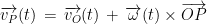
dove O è un altro punto del corpo (o dello spazio solidale ad esso) e dove $\overrightarrow{\omega}$ è la velocità angolare (vedi qui, cap IV). Ora, se si prende la curva per P la cui tangenete è $\overrightarrow{v_P}(t)$ e la si prolunga in modo che sia tangente in ogni suo punto al valore del campo delle velocità in quello stesso punto, si ottiene una elica, comunque si scelga P (Figura 1). L’elica cioè descrive proprio la matrice matematica del moto dei corpi nello spazio, oltre ad essere, come visto, una costante nelle forme naturali, microscopiche, nanoscopiche, e macroscopiche. E sebbene queste nozioni di cinematica siano posteriori ai Philosophiae Naturalis Principia Mathematica (1687), gli artisti hanno sempre usato l’elica esattamente per suggerire una idea di moto, senza contare il fatto che l’elica sembra anche inscrivere in sé ulteriori connotazioni emotive e significati. L’elica, che non ha piani di simmetria (sebbene abbia punti di simmetria), è stata usata per animare le forme simmetrche, a un certo punto della storia dell’arte, essendo la simmetria forse il criterio di bellezza originario, quello a cui allude il poeta-pittore William Blake: “What immortal hand or eye could frame thy fearful simmetry?” (The Tyger, 1794).

Figura 1. Due curve tangenti, punto per punto, al medesimo campo vettoriale elicoidale. Il codice che genera questa figura è in appendice (risolve numericamente un sistema di tre equazioni differenziali). Sono indicati anche i versori del campo elicoidale per alcuni dei punti delle curve.

Io stesso tendo ad usare la torsione nelle mie composizioni: in Figura 2, il personaggio di spalle ha la testa che punta verso destra, mentre i suoi piedi si intuisce puntino a sinistra; dunque attraverso la sua lunghezza si realizza una rotazione del piano coronale (o frontale) di quasi 90°.

Figura 2. “*You can’t win”, matita su carta, di Paolo Maccallini. Il disegno è ancora incompleto.*

3. Creatori di mostri

Il Laocoonte dunque nasce una seconda volta nel 1506. Ma cosa si può dire della sua vera nascita? Tralasciando il dibattito sulla presunta presenza di un originale in bronzo più antico di un secolo, siamo davanti all’intrigante questione del rapporto tra la statua e i versi 201-224 del secondo libro della Eneide, che seguono la medesima narrazione. Virgilio scrisse l’Eneide tra il 29 e il 19 a.C.; il gruppo marmoreo fu prodotto tra il 40 e il 20 dello stesso secolo. Chi ha ispirato chi? Immagino che questa sia una domanda formulata più volte da menti ben più preparate della mia in questo genere di esercizi; io osservo solo che mentre Virgilio preferisce dei mostri (li chiama angues, serpens, dracones) che non hanno una corrispondenza con la zoologia nota (dimensioni a parte, sono serpenti con creste vermiglie: iubaeque sanguineae exsuperant undas), gli autori di Rodi decidono di seguire pedissequamente la natura, usando due pitoni, o qualcosa di molto simile a questo serpente africano, probabilmente non sconosciuto alle culture mediterranee. Riflettendo sulla scelta dei tre scultori, mi sono venute in mente le parole del costruttore di mostri per eccellenza, l’inventore della meccatronica applicata al cinema, Carlo Rambaldi, il quale in un libro del 1987 dice:

Se cerchi di andare al di là della natura e realizzare una cosa assolutamente fantastica, sei libero di fare quello che vuoi; ma se devi imitare la natura – e l’abbiamo sperimentato più volte – conviene guardare la natura.
Leonardo Pellizzari (a cura di), Carlo Rambaldi e gli Effetti Speciali, 1987

Si può dire certo che le creste non sarebbe stato possibile renderle in marmo, ed è vero probabilmente, tuttavia sono convinto che i tre di Rodi abbiano seguito il percorso mentale di Rambaldi; traiettoria che anche io, nei miei tentativi di disegno e nei miei sogni ingegneristici, ho preconizzato. Altrimenti detto: la Natura ha sempre più fantasia degli esseri umani. E la investigazione scientifica non ha fatto che confermarmi questa intuizione.

Segue la mia traduzione, in endecasillabi, dei versi di Virgilio menzionati sopra, e in appendice trovate il computo delle sillabe, i versi originali, la parafrasi in latino e la traduzione letterale.

Assegnato al culto del dio Nettuno
Laocoonte un degno toro offriva.
Ma da Tenedo adesso le calme acque
sovrastano immensi due serpenti
che speculari puntano la costa,
i colli eretti tra i flutti, vermiglie
le creste sopra le onde, immensa mole
del corpo si snoda, e sfiora il mare.
Scroscio di schiuma, e sono sulla riva,
gli occhi iniettati di sangue di fuoco,
lingue vibranti e labbra sibilanti.
Fuggiamo, a Laocoonte aspirano,
ma prima i piccoli corpi dei figli
ambedue i serpenti avvolti stringon
e ingoiano i morsi dei miseri arti.
Poi assalgono il padre accorso in aiuto
armato che nelle spire è legato;
e già su di lui torreggiano, stretto
due volte il busto, per due il collo avvinto. 
Mentre tenta di liberare i nodi,
le vesti pregne di bava letale,
grida disumane lancia alle stelle,
qual mugge il toro che l'altare fugge
scuotendo il collo, la malferma scure.

4. L’antidoto

Il Laocoonte, di marmo o di versi, è dunque la rappresentazione della sofferenza senza luce: una famiglia è spazzata via con una agonia inimmaginabile, quella del cervo mangiato vivo dal predatore, con l’aggravante della consapevolezza della morte. E poi c’è un dolore ancora più grande, inconcepito, innominabile forse: quello della moglie e madre.

Laocoonte, che qualche verso prima tentava di avvisare i troiani sulla pericolosità del cavallo di legno (“timeo Danaos et dona ferentes”), è la voce della ragione davanti al destino oscuro dell’uomo, quello di finire nel gorgo e scomparire; i troiani sono la voce della speranza, che rischia di cadere in trappola (lo vediamo nel fiorire della medicina alternativa per le malattie senza cura e nelle promesse di resurrezione dei vari culti). E’ l’islandese di Leopardi, la voce di Tolstoj in “Confessione”. E’ quello che resta, al netto delle religioni orientali che vennero dopo il mondo pagano, come antidoto. Non è un caso che Stefano Benni posizioni una copia di questa statua nella dimora del suo Achille pié veloce. Eppure nella statua stessa, nel monumento alla cognizione del dolore, c’è un antidoto: la creazione superba, la maestria, il talento strabordante, lo studio minuto della Natura. Il Laocoonte è esso stesso l’antidoto al veleno, sia nel marmo che nei versi. Ed è per questo che menziono nel titolo e nel testo il volume di Gadda: la sua Cognizione del Dolore, con la morte del fratello, la vecchiezza della madre vedova poi uccisa, la follia lucida del figlio che forse assassina la madre (forse no, c’è un indizio nel romanzo), è completamente priva di assoluzione, di resurrezione; se non nel virtuosismo linguistico e nell’analisi della natura umana. Sono opere queste che mostrano l’abisso e allo stesso tempo vi costruiscono sopra un ponte.

Figura 3. *Baccio Bandinelli, Laocoonte, 1520-1525, Galleria degli Uffizi.* *Foto di Paolo Maccallini.*

La foto che ho usato in Figura 3 non è del Laocoonte di Agesandro, Polidoro e Atenodoro, lo so. Non si tratta di un errore. La statua degli scultori di Rodi la trovate con la ricerca per immagini su Google, amesso che non sia scolpita nella vostra mente. Questo Laocoonte è la copia di Baccio Bandinelli, un artista che fu costretto dalla committenza e dalle circostanze temporali ad affrontare un gigante sul suo stesso terreno di battaglia: dovette competere con Michelangelo nella statuaria monumentale a tutto tondo, e perse tragicamente. La sua copia del Laocoonte è forse la sua statua più riuscita, se si escludono i bassorilievi per i quali aveva probabilmente più talento. Io ho conosciuto Bandinelli grazie a questa statua, che mi trovai un giorno al fondo della prospettiva di un corridoio degli Uffizi, che arrotolavo come un nastro sotto la mia sedia a rotelle, in una foresta di gambe in passeggio aleatorio.

5. Appendice

Di seguito riporto il conteggio delle sillabe per la mia traduzione, tenendo conto delle sinalefe.

as	se	gna	toal	cul	to	del	dio	Net	tu	no
La	o	co	on	te	de	gno	to	roof	fri	va
ma	da	Te	ne	doa	des	so	le	cal	meac	que
so	vra	sta	noim	men	si	du	e	ser	pen	ti
che	spe	cu	la	ri	pun	ta	no	la	cos	ta
i	col	lie	ret	ti	trai	flut	ti	ver	mi	glie
le	cre	ste	so	pra	leon	deim	men	sa	mo	le
del	cor	po	si	sno	dae	sfio	ra	il	ma	re
scro	scio	di	schiu	mae	so	no	sul	la	ri	va
glioc	chii	niet	ta	ti	di	san	guee	di	fuo	co
lin	gue	vi	bran	tie	lab	bra	si	bi	lan	ti
fug	gia	moa	la	o	co	on	tea	spi	ra	no
ma	pri	mai	pic	co	li	cor	pi	dei	fi	gli
am	be	du	ei	ser	pen	tiav	vol	ti	strin	gon
ein	go	ia	noi	mor	si	dei	mi	se	riar	ti
poias	sal	go	noil	pa	dreac	cor	soin	a	iu	to
ar	ma	to	che	nel	le	spi	reè	le	ga	to
e	già	su	di	lui	tor	reg	gia	no	stret	to
due	vol	teil	bu	sto	per	dueil	col	loav	vin	to
men	tre	ten	ta	di	li	be	ra	rei	no	di
le	ves	ti	pre	gne	di	ba	va	le	ta	le
gri	da	di	su	ma	ne	lan	ciaal	le	stel	le
qual	mug	geil	to	ro	che	lal	ta	re	fug	ge
scuo	ten	doil	col	lo	la	mal	fer	ma	scu	re

L’intero secondo libro della Eneide in latino si trova qui. In particolare, i versi tradotti sono i seguenti.

Laocoon, ductus Neptuno forte sacerdos,
solemnes taurum ingentem mactabat ad aras. 
Ecce autem gemini a Tenedo tranquilla per alta
(horresco referens) immensis orbibus angues
incumbunt pelago, pariterque ad litora tendunt:
pectora quorum inter fluctus arrecta, iubaeque
sanguineae exsuperant undas: pars cetera pontum
pone legit, sinvatque immensa volumine terga.
Fit sonitus spumante salo: iamque arva tenebant,
ardentesque oculos suffecti sanguine, et igni,
sibila lambebant linguis vibrantibus ora.
Diffugimus visu exsangues: illi agmine certo
Laocoonta petunt, et primum parva duorum
corpora natorum serpens amplexus uterque
implicat, et miseros morsu depascitur artus.
Post ipsum auxilio subeuntem ac tela ferentem
corripiunt spirisque ligant ingentibus; et iam
bis medium amplexi, bis collo squamea circum
terga dati, superant capite et cervicibus altis.
Ille simul manibus tendit divellere nodos
perfusus sanie vittas atroque veneno;
clamores simul horrendos ad sidera tollit,
quales mugitus, fugit cum saucius aras
taurus et incertam excussit cervice securim.
At gemini lapsu delubra ad summa dracones
effugiunt, saevaeque petunt Tritonidis arcem,
sub pedibusque deae, clypeique sub orbe teguntur.

Di seguito le medesime parole, disposte nella costruzione italiana, con una traduzione parola per parola.

Laocoon, ductus sacerdos Neptuno forte, mactabat ingentem taurum ad aras solemnes.

Laocoonte, nominato sacerdote di Nettuno per sorteggio, uccideva un grande toro presso i solenni altari.

Ecce autem a Tenedo per alta tranquilla [aequora] angues gemini (horresco referens) incumbunt pelago immensis orbibus, pariterque tendunt ad litora:

Ma ecco che da Tenedo, attraverso le acque tranquille, due serpenti gemelli (inorridisco nel raccontarlo) sovrastano il mare con le spire immense, e puntano la riva all’unisono:

pectora quorum arrecta [sunt] inter fluctus, iubaeque sanguineae exsuperant undas: pars cetera legit pontum, pone, sinvatque volumine immensa terga [= terga immenso volumine, ipallage].

i petti dei quali sono eretti sui flutti, e le creste vermiglie si innalzano oltre le onde: il resto del corpo sfiora il mare, dietro, e snoda il dorso in immense spire.

Sonitus fit salo spumante: iamque tenebat arva et, oculos ardentes [acc. di rel.] suffecti sanguine et igni, lambebant sibila ora linguis vibrantibus.

Un gorgoglio è generato dalla mare spumeggiante: già avevano raggiunto la costa e, con occhi ardenti iniettati di sangue e fuoco, lambivano le bocche sibilanto con lingue vibranti.

Diffugimus exangues visu: illi petunt Laocoonta, agmine certo, et primum uterque serpens amplexus implicat parva corpora duorum natorum, et depascitur miseros artus morsu.

Scappiamo con visi esangui: essi puntano Laocoonte, con andatura decisa, e prima i due serpenti stringono, avvolti, i piccoli corpi dei due figli, e divorano i miseri arti a morsi.

Post corripiunt ipsum [Laocoonta], auxilio subeuntem ac tela ferentem, et ligant spiris ingentibus;

Quindi assalgono lo stesso Laocoonte, che accorre in soccorso e porta delle armi, e lo avvincono con le ingenti spire;

et iam amplexi bis medium [acc. di rel.], circumdati [timesi] squamea terga [acc. di rel.] bis collo, superant altis capite et cervicibus.

e stretto due volte il busto [di Laocoonte], due volte avvolte intorno al collo le terga squamose, già torreggiano con il collo e il capo.

Ille simul tendit divellere nodos manibus, vittas perfusus [acc. alla greca] sanie et atro veneno; simul tollit horrendos clamores ad sidera:

Lui, con le bende imbevute di bava e veleno nero, tenta di sciogliere i nodi con le mani mentre leva orrende grida al cielo,

quales mugitus taurus [tollit], cum fugitsaucius aras, et excussit incertam securim cervice.

come i muggiti del toro che fugge ferito dall’altare mentre si squote dal collo la scure malferma.

At gemini dracones effugiunt lapsu ad summa delubra, et petunt arcem saevae Tritonidis, et teguntur sub pedibus deae, et sub orbe clypei.

E i draghi gemelli fuggono strisciando verso gli alti santuari, e si dirigono all’altare della ostile Tritonia [Atena], e si nascondono sotto i piedi della dea, sotto il cerchio dello scudo.

Di seguito il codice in Octave che genera Figura 1, risolvendo numericamente (metodo di Runge-Kutta) il sistema di tre equazioni differenziali ordinarie seguente:

Eq. 2) $\begin{cases}\frac{dx(s)}{ds}\,=\,\tau_{x}(s)\\\frac{dy(s)}{ds}\,=\,\tau_{y}(s)\\\frac{dz(s)}{ds}\,=\,\tau_{z}(s)\end{cases}$

dove $\overrightarrow{\tau}$ è il versore relativo al campo vettoriale in Eq. 1. Il codice funziona qualunque sia il campo vettoriale inserito nella funzione interna allo script (vectorial_field). Ho scritto questo codice nel 2021, come dimostrazione del metodo di ricostruzione delle fibre di materia bianca nella risonanza magnetica cerebrale con trattografia (Maccallini P. 2021).

% file name = tractography
% date of creation = 05/02/2021
% it plots the trajectory of a fibre, given a vectorial field of diffusion
% eigenvector epsilon_1
clear all
close all
% vectorial field
v = [0,0,3];
w = [0,0,3];
ic = [1.5,1.5,0];
delta_s = 0.5;
function v_f = vectorial_field (x,y,z,v,w)
  v_f = v + cross(w,[x,y,z]);
  v_f = v_f/sqrt(v_f(1)^2+v_f(2)^2+v_f(3)^2);
endfunction
% we set the initial conditions for the first fiber
lambda(1:4,1:3)=0.;
x(1) = ic(1);
y(1) = ic(2);
z(1) = ic(3);
% integration for the first fiber
vector = vectorial_field (x(1),y(1),z(1),v,w);
lambda(1,1) = vector(1);
lambda(1,2) = vector(2);
lambda(1,3) = vector(3);
n = 40;
for i=1:n-1
  for k=2:4
    vector = vectorial_field (x(i)+lambda(k,1)*delta_s/2,y(i)+lambda(k,2)*delta_s/2,z(i)+lambda(k,3)*delta_s/2,v,w);
    lambda(k,1) = vector(1);
    lambda(k,2) = vector(2);
    lambda(k,3) = vector(3);
  endfor
  x(i+1) = x(i)+(lambda(1,1)+2*lambda(2,1)+2*lambda(3,1)+lambda(4,1))*delta_s/6;
  y(i+1) = y(i)+(lambda(1,2)+2*lambda(2,2)+2*lambda(3,2)+lambda(4,2))*delta_s/6;
  z(i+1) = z(i)+(lambda(1,3)+2*lambda(2,3)+2*lambda(3,3)+lambda(4,3))*delta_s/6;
  vector = vectorial_field (x(i+1),y(i+1),z(i+1),v,w);
  quiver3 ( x(i+1),y(i+1),z(i+1),vector(1),vector(2),vector(3),'-k' )
  hold on
endfor
plot3 (x(1:n),y(1:n),z(1:n),'-r','LineWidth',4)
pbaspect ([1, 1, 1])
hold on
% we set the initial conditions for the second fiber
ic = [2.8,2.8,0];
x(1) = ic(1);
y(1) = ic(2);
z(1) = ic(3);
% integration for the second fiber
vector = vectorial_field (x(1),y(1),z(1),v,w);
lambda(1,1) = vector(1);
lambda(1,2) = vector(2);
lambda(1,3) = vector(3);
for i=1:n-1
  for k=2:4
    vector = vectorial_field (x(i)+lambda(k,1)*delta_s/2,y(i)+lambda(k,2)*delta_s/2,z(i)+lambda(k,3)*delta_s/2,v,w);
    lambda(k,1) = vector(1);
    lambda(k,2) = vector(2);
    lambda(k,3) = vector(3);
  endfor
  x(i+1) = x(i)+(lambda(1,1)+2*lambda(2,1)+2*lambda(3,1)+lambda(4,1))*delta_s/6;
  y(i+1) = y(i)+(lambda(1,2)+2*lambda(2,2)+2*lambda(3,2)+lambda(4,2))*delta_s/6;
  z(i+1) = z(i)+(lambda(1,3)+2*lambda(2,3)+2*lambda(3,3)+lambda(4,3))*delta_s/6;
  vector = vectorial_field (x(i+1),y(i+1),z(i+1),v,w);
  quiver3 ( x(i+1),y(i+1),z(i+1),vector(1),vector(2),vector(3),'-k' )
  hold on
endfor
plot3 (x(1:n),y(1:n),z(1:n),'-b','LineWidth',4)
pbaspect ([1, 1, 1])
grid on

Summer simulation, a correlation study

Abstract

I report here on a successful attempt at reproducing the improvement in my ME/CFS symptoms that I usually experience during summer by means of artificially manipulating the temperature of the air, humidity, and the infrared radiation inside a room I spent five months in, during the period from December to April 2022. I show that the improvement is not correlated with the physical parameters of the air (temperature, relative and absolute humidity, atmospheric pressure, air density, dry air density, saturation vapor pressure, and partial vapor pressure). I hypothesize that it is driven instead by either the mid-wave infrared radiation emitted by a lamp used in the experiment or by the longwave infrared radiation emitted by the walls of the room in which I spent the months of the experiment.

1) Introduction

My ME/CFS improves during summer, in the period of the year that goes from May/June to the end of September (when I am in Rome, Italy). I don’t know why. In a previous study (Maccallini P. 2022), I analyzed the correlation between my symptoms and several environmental parameters, during three periods covering a total of 190 days: in one, I improved while the season was going toward summer, in another one we were in full-blown summer, and in the third one my functioning declined while summer was fading away. The statistical analysis showed a positive correlation between my functionality score and the temperature of the air and a negative correlation between my functionality score and air density and dry air density (remember that the higher the functionality score, the better I feel). No correlation was found between my functionality score and: relative humidity, absolute humidity, atmospheric pressure, and the concentration of particulate with a diameter below or equal to $2.5\,\mu m$ . 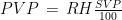While the absence of correlation can be used to rule out causation, the presence of correlation does not mean automatically causation. Moreover, since air density and dry air density are strongly inversely correlated with air temperature, the correlations with air density might be driven by the correlation with air temperature (and vice-versa). In order to further investigate the nature of these correlations, I planned a second study, this time performed inside a chamber where I could manipulate the temperature of the air, the content of water in the air, and the amount of infrared radiation I was hit by. I called this chamber “Summer Simulator” because I used several devices to obtain, during the months from December to May, the conditions that we usually have in Rome during summer. I lived inside the simulator while I collected a functionality score, three times per day, and while I measured (every 10 minutes) the temperature of the air, relative humidity, and atmospheric pressure. The data for the months from January to April were used to study how my symptoms correlated with the environmental parameters I could directly measure and those that I could mathematically derive.

2) Methods

2.1) Data collection

I used a Bresser WiFi 4-in-1 Weather Station (see figure 1) to measure the temperature of the air, pressure, and relative humidity inside the room I spent almost all my time during the experiment. Measures were registered every 10 minutes and sent to the console which uploaded them to my Weathercloud account, via WiFi. The barometer was calibrated by using the closest weather station of the meteorological network of Rome (R). I registered a functionality score three times a day (value from 3 to 7, the higher the better) to use for the search for correlations with environmental data. The data that were employed were those of January, February, March, and April 2022. I also used the daily functionality score collected in 2017, during the same months, for testing the effect of the Summer Simulator on my symptoms.

Figure 1. Bresser 4-in-1 sensor: I used it to measure the temperature of the air, atmospheric pressure, and relative humidity inside the simulator. In the second image, you see the interface of the weather station (left) and a CO2 sensor I used to ensure that the air exchange in the room was adequate.

2.2) Summer Simulator

Simulation of summer was attempted with the following settings. I lived for 5 months in a room of $9\,m^2$ . The temperature was controlled by a heat pump (Electrolux EXP26U558HW) that collects air from inside the room, divides it into two fluxes, transfers heat from one to the other (by cycles of compression-evaporation of refrigerant R290), and releases the warmer flux inside and the other one outside the window. The humidity was controlled by two/three ultrasonic mist humidifiers that release mist which is then turned into vapor in a fraction that depends on the temperature of the air (Figure 2).

**Figure 2**. Ultrasonic mist humidifiers.

To simulate thermal radiation, I used an infrared heater (Turbo TN35E, figure 3) coupled with a chamber with walls covered by mylar, a material that reflects most of the thermal radiation; the chamber was built around the bed, and it had only one side open, to allow for air circulation (figure 4).

**Figure 3**. Infrared heater, Turbo TN35E.

Figure 4. The infrared chamber with walls made up of mylar, a material that reflects thermal radiation. On the right, you can see the heat pump (white) and the pipeline of the exhausted air, behind the curtain, that leads outside, through a hole in the window.

The infrared heater was, on average, at a distance of 0.8 m from the left side of the bed. It emits most of its power in the mid-wave infrared range (1-4 $\mu m$ ).

2.3) Mathematical model for the infrared radiation

I built a mathematical model for the radiation from the lamp (Maccallini P. 2022) which predicts that the power per unit of area of a plane parallel to yz (see figure 4) centered in $P\equiv(x_P,\,y_P,\,z_P)$ is given by

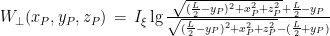
1) $W_\bot(x_P, y_P,z_P)\,=\,I_\xi\lg{\frac{\sqrt{(\frac{L}{2}-y_P)^2+x_P^2 +z_P^2 }+\frac{L}{2}-y_P}{\sqrt{(\frac{L}{2}-y_P)^2+x_P^2 +z_P^2 }-(\frac{L}{2}+y_P)}}$

where L = 0.53 m is the length of the emitting surface of the lamp on the y axis and where

2) $I_\xi\,=\,\frac{e\Pi(1-4b^2)\sqrt{1-4c^2}}{8\pi hLbc[F(\arctan\sqrt{\frac{1-4c^2}{4c^2}},\sqrt{\frac{1-4b^2}{1-4c^2}})-E(\arctan\sqrt{\frac{1-4c^2}{4c^2}},\sqrt{\frac{1-4b^2}{1-4c^2}})]}$

In this formula, e is the efficiency of the conversion of electrical power into mid-wave infrared emission (it is 93% according to the manufacturer) while $\Pi$ is the power absorbed by the device (about 800 W, according to the measurements performed by a power meter) and where F and E are the elliptic functions of the first and second kind, respectively (Maccallini P 2013). Parameters b and c (the semi-axes of the ellipsoid in figure 5, in the directions y and z, respectively) depend on how the flux of radiant power is concentrated by the reflector of the lamp. In my model, they are undetermined and must be derived by a minimum of two independent measures of power per unit area. But in the absence of these measures, we can use the values for which we have the absolute minimum for the function $I_\xi (b, c)$ which is reached for b = 0.49, c = 0.36 (assuming c < b < 0.5).

Figure 5. On the left, the systems of coordinates used for building the mathematical model of the infrared heater. On the right, the detail of the ellipsoid that describes the concentration of the radiant power that exits the heater as a result of the power released by the bulb and the power reflected by the reflector behind the bulb; this ellipsoid is represented as a sphere on the left side of this figure. All the details of the model can be found in (Maccallini P. 2022).

The solution of the model (equations 1 and 2) was determined analytically, the values for the elliptic functions were calculated by employing Wolfram Mathematica 5.2 as a function of b and c and saved in a csv file, then the output of the lamp was calculated by a custom script written in Octave (Maccallini P. 2022) that used the output from the Mathematica script. Note that Octave does not have a built-in function for the elliptic functions and a numerical integration by Simpson’s rule led to unsatisfactory results, as detailed in the already mentioned reference. The prediction for a plane parallel to yz at a distance $x_P\,=\,0.8\,m$ from O, is reported in figure 6, where it can be seen that the maximum of $W_\bot$ is reached for $P\equiv(0.8,\,0,\,0)$ and its value is about 376 $\frac{W}{m^2}$ .

Figure 6. The power per unit of area orthogonal to the plane zy ( $W_\bot$ ), as a function of $x_P, y_P, z_P$ , for $x_P\,=\,0.8\,m$ .

2.4) Derived environmental parameters

The weather station only measured air temperature, atmospheric pressure, and relative humidity, every 10 minutes. The measures were then uploaded via WiFi to a server and downloaded to my computer from my Weathercloud account. To calculate the daily means of these parameters I designed an algorithm that takes into account missing data, as follows: it calculates an hourly mean measure when at least one measure is available for that hour; it fills isolate missing hourly means with the mean between the measure of the hour before and the one of the following hour; it then calculates the daily mean if the hourly means of at least 21 hours are present for each day, otherwise the daily mean is considered as a missing value. From the hourly means of temperature, relative humidity, and pressure, I calculated the hourly means for saturation vapor pressure (SVP), partial vapor pressure (PVP), absolute humidity (AH), dry air density (DAD), and air density (AD), by means of the following formulae:

3) $SVP\;=\;6.112e^{\frac{17.62t}{243.12+t}}$

4) $PVP\,=\,RH\frac{SVP}{100}$

5) $AH\,=\,100\mu_w\frac{PVP}{R(273.15\,+\,t)}$

6) $DAD\,=\,100\mu_{dry}\frac{p\,-\,PVP}{R(273.15\,+\,t)}$

7) $AD\,=\,AH\,+\,DAD$

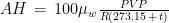
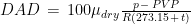
where t, p, RH are air temperature, barometric pressure, and relative humidity, respectively, while $\mu_w\,=\,18.015\frac{g}{mol}$ is the molecular weight of water, $\mu_{dry}\,=\,28.97\frac{g}{mol}$ is the molecular weight of dry air, $R\,=\,8.31\frac{J}{K\cdot mol}$ is the constant of gasses, and where we express temperature in °C and pressure in hPa. These formulae are taken from chapter 4 of the Guide to Instruments and Methods of Observation by the World Meteorological Organization (R) and are derived and discussed in (Maccallini P. 2021). Once obtained the hourly means for the derived environmental measures, the corresponding daily means were computed by using the same method described for t, p, and RH. In figure 8, I reported, as an example, the plots for the environmental parameters (daily means) and the mean daily score for the month of March. All the other plots can be obtained by running the R script reported at the end of this article, in the same folder containing the raw data (that are available, just before the script, for download).

2.5) Statistical analysis

To assess the effect of the summer simulation on my symptoms, I compared the functionality score collected in 2017 (from January to April) with the score collected during the same months of 2022, while living inside the Summer Simulator. The null hypothesis was tested by running the Wilcox test. The correlations between the daily mean score and the environmental parameters were assessed by Spearman’s correlation coefficient and the significance of each correlation was also tested. All the calculations were performed by a custom R script written by myself, available, along with the row data, at the bottom of this page.

3) Results

The comparison between the mean daily scores for the months of January, February, March, and April 2017 and the same parameter for the same months of the year 2022 show that the Summer Simulator has raised the mean daily score in a statistically significant fashion: p value = $1.897\cdot10^{-10}$ ; see figure 7.

Figure 7. Comparison between the mean daily functionality score in 2017 (from January to April), on the right, and the same score in 2022 (same months), while living inside the Summer Simulator, on the left. The difference is statistically significant, reaching a p value of $1.897\cdot10^{-10}$ . In 2017 I was following a therapy that I judged mildly effective, which allowed me to take the functionality score three times a day during the cold months, which is something that I usually stop doing when I get worse in Autumn, also because the score would always be the lowest one. The diagram is a box and whisker plot, with the indication of the 1st quantile, the median (2nd quantile), and the 3rd quantile.

Figure 8. Daily mean values for each one of the environmental parameters considered in this study and for the functionality score, for the month of March.

The correlations between the mean daily score and the mean daily values of the environmental parameters, and the corresponding p values, are collected in Table 1. After correction for multiple comparisons (Benjamini-Hochberg method), none of the correlations reaches statistical significance.

Table 1. Correlations between the mean daily functionality score and several environmental parameters (Spearman’s rank correlation coefficient) and the corresponding p values before and after correction for multiple comparisons (Benjamini-Hochberg method).

I run a similar analysis with another method, too: I compared the daily mean temperatures for days with a mean functionality score above 5 and the daily mean temperature for the days with a score below 5, by running the Wilcox test; I repeated this same analysis for all the other environmental parameters (see Table 2 and figure 8).

Figure 8. For each environmental parameter, you find here the comparison between the mean daily value corresponding to days with a mean functionality score above 5, equal to 5, and below 5. Box and whisker plots, with also the indication of the means, as red dots. The p values for the comparisons between days with a mean functionality score below 5 and above 5 are collected in table 2.

Parameter	p	p‘
Temperature	0.02694	0.1813
Relative humidity	0.133	0.2112
Pressure	0.2112	0.2112
Saturation vapor pressure	0.02535	0.1813
Partial vapor pressure	0.06324	0.1897
Absolute humidity	0.06213	0.1897
Dry air density	0.03038	0.1813
Air density	0.03625	0.1813

Table 2. For each environmental parameter, I compared the daily mean value corresponding to days with a functionality score above 5, with the same value for days with a functionality score below 5 (Wilcox test) and I corrected for multiple comparisons (Benjamini-Hochberg method).

4) Discussion

Simulation of summer by raising the air temperature, absolute humidity, and infrared radiation did show to improve my symptoms when I compared my daily functionality score with the score collected for the same period of the year, but in 2017, while I was following another therapy that I judged mildly effective (figure 7). Yet, no correlation reached statistical significance between my functionality score and the environmental parameters that could be measured or derived (temperature, relative and absolute humidity, atmospheric pressure, saturation vapor pressure, partial vapor pressure, dry air density, air density). If we accept that the summer simulation has really improved my condition (i.e. if we rule out a placebo effect), we must admit that the improvement was due to either some combination of the aforementioned parameters or something else. The only other parameter I could exert my control on was infrared radiation by an infrared heater that delivered a power of about $380\,\frac{W}{m^2}$ on the vertical plane by the left side of my bed, according to a mathematical model of the lamp (figure 6). This radiation was then partially reflected by the surfaces covered in mylar of my infrared chamber, so that it hit my body from other directions too, even though I have not built a model for the whole infrared chamber, yet.

One possible explanation, to my understanding, for the results of this study, is then that the improvement was driven by some effect of the radiation from the lamp, either directly on my body or indirectly to some other parameter of the environment which in turn affected my biology. Importantly, the absence of correlation with air temperature, air density, and dry air density reported by the present study suggests that the significant correlations found in the previous study (Maccallini P. 2022) between my functionality score and the three mentioned parameters were driven by something else that correlates with temperature (which negatively correlates with air density and dry air density). We know that there is an almost linear positive correlation between the temperature of the air and longwave infrared radiation from the Earth into space (Koll DDB and Cronin TW 2018), while the emission of the surface of the Earth within a short distance from it must follow the Stefan-Boltzman law so that it is proportional to $T^4$ , where T is the temperature of the air at the level of the surface, expressed in Kelvin. But it should be noted that while 99% of the power emitted by the Earth as infrared radiation has a wavelength above $5\,\mu m$ , my infrared heater emits in the range $1-4\,\mu m$ . So, my artificial source of radiation does not simulate the radiation from the Earth, if we consider the wavelength (while it does from the point of view of the total power, as we will see in a following study, already concluded). But it could be considered that the radiation from the lamp did end up hitting the walls of my room, which in turn released their thermic energy as long wave infrared radiation. It is conceivable then that both in the Summer Simulator and in real summer, my improvements might be driven by far infrared radiation. Another possibility is that the improvement was due to the infrared radiation emitted by my body (long wave infrared radiation) and reflected back to me by the mylar coating of the infrared chamber.

I can’t rule out a placebo effect of the Summer Simulator, even though it showed greater effectiveness than another therapy I was following in 2017, which I considered mildly effective. The difficulty of assessing the effectiveness of a treatment by a subjective score can hardly be overestimated. The identification of objective measures that can be routinely used to score the level of symptoms is of paramount importance for correlation studies like the present one.

5) Conclusions

By simulating summer during the months from January to April of 2022, I experienced an improvement in my symptoms similar to the one I usually experience during summer (although of a lesser magnitude). The simulation was achieved by increasing air temperature and absolute humidity, by using an infrared heater, and by living inside a chamber covered with mylar, a material that reflects most of the thermal radiation, so to avoid dispersion of the radiation from the heater. The improvement does not correlate with any of the parameters of the air (temperature, absolute and relative humidity, saturation vapor pressure, partial vapor pressure, density of the air, density of dry air, atmospheric pressure). One possible explanation for my improvement while living inside the Summer Simulator is that it was due to either the direct radiation from the heater (which is mid-wave infrared radiation) or the radiation from the walls heated by the lamp and the air. The latter radiation is far infrared radiation, the same radiation emitted by the Earth, which linearly correlates with air temperature and which might drive the improvements I experience during summer and the correlation between my functionality score and air temperature reported in a previous study.

6) Funding

This study was supported by those who donated to this website.

7) Supplementary material

The environmental measures and the symptom scores used for this study are available for download:

Score_control_Summer_Simulator.csv

Score_Summer_Simulator.csv

Weathercloud_2022_1.csv

Weathercloud_2022_2.csv

Weathercloud_2022_3.csv

Weathercloud_2022_4.csv

The mathematical model of the infrared heater is available here for download. The script I wrote in R for the statistical analyses is the following one.

# file name: summer_simulator
#
# year: 2022
# month: 08
# day: 31
#
#-------------------------------------------------------------------------------
# We read the measures from Bresser Weather Station
#-------------------------------------------------------------------------------
#
# We set the names of the columns for the data.frames containing environmental data
#
cn<-c("Date","Tempin","Temp","Chill","Dewin","Dew","Heatin","Heat","Humin","Hum",
      "Wspdhi","Wspdavg","Wdiravg","Bar", "Rain", "Rainrate","Solarrad","Uvi")
#
# We read the environmental data
#
Jan_2022<-read.csv("Weathercloud Paolo WS 2022-01.csv", sep = ";", col.names = cn, header = T)
Feb_2022<-read.csv("Weathercloud Paolo WS 2022-02.csv", sep = ";", col.names = cn, header = T)
Mar_2022<-read.csv("Weathercloud Paolo WS 2022-03.csv", sep = ";", col.names = cn, header = T)
Apr_2022<-read.csv("Weathercloud Paolo WS 2022-04.csv", sep = ";", col.names = cn, header = T)
List_2022<-list(Jan_2022, Feb_2022, Mar_2022, Apr_2022)
#
# We set some parameters
#
mis<-3 # the highest number of missing hours accepted for a day
muw<-18.01528 # molecular weight of water (g/mol)
mud<-28.97 # molecular weight of dry air (g/mol)
R<-8.31 # universal constant of gasses (J/(K*mole))
month_name<-c("January", "February", "March", "April")
#
#-------------------------------------------------------------------------------
# We work on the score
#-------------------------------------------------------------------------------
#
# We set the names of the columns for the data.frame containing the score
#
cn<-c("Year","Month","Day","score_1","score_2","score_3")
#
# We read the scores
#
Score<-read.csv("Score_Summer_Simulator.csv", sep = ";", col.names = cn, header = T)
Score_control<-read.csv("Score_control_Summer_Simulator.csv", sep = ";", col.names = cn, header = T)
#
attach(Score)
#
ms<-c(rep(0,31*4))
#
# We calculate the daily mean score
#
for (d in 1:length(Year)) {
  if (is.na(score_1[d])==F&is.na(score_2[d])==F&is.na(score_3[d])==F) {
    ms[d]<-(score_1[d] + score_2[d] + score_3[d])/3  
  } else ms[d]<-NA
}
#
attach(Score_control)
#
ms_c<-c(rep(0,length(Year)))
#
# We calculate the daily mean score
#
for (d in 1:length(Year)) {
  if (is.na(score_1[d])==F&is.na(score_2[d])==F&is.na(score_3[d])==F) {
    ms_c[d]<-(score_1[d] + score_2[d] + score_3[d])/3  
  } else ms[d]<-NA
}
#
# We test the effect of the simulator 
#
wilcox.test(ms, ms_c)
boxplot(ms, ms_c, ylab = "score", names = c("summer simulator","other"))
#
#-------------------------------------------------------------------------------
# We calculate mean values for temp (°C), relative humidity (%), and atmospheric 
# pressure (hPa) 
#-------------------------------------------------------------------------------
#
# We initialize the arrays that will contain the daily means of the environmental 
# data
#
t<-c(rep(0,31*4))
rh<-c(rep(0,31*4))
p<-c(rep(0,31*4))
svp<-c(rep(0,31*4))
pvp<-c(rep(0,31*4))
ah<-c(rep(0,31*4))
dad<-c(rep(0,31*4))
ad<-c(rep(0,31*4))
#
#-------------------------------------------------------------------------------
# We work on each month
#-------------------------------------------------------------------------------
#
for (q in 1:4) {
  index<-q
  add<-31*(q-1)
  attach(List_2022[[q]])
  #
  # We extract the day of the month, the year, the hour from column Date
  #
  DateR<-read.table(text=Jan_2022[,1], sep ="/")
  DateR2<-read.table(text=DateR[,3], sep =" ")
  DateR3<-read.table(text=DateR2[,2], sep =":")
  #
  #-------------------------------------------------------------------------------
  #
  first_day<-DateR[1,1]
  last_day<-DateR[length(DateR[,1]),1]
  #
  # We calculate the hourly mean for temperature (°C)
  #
  Temp_mean<-matrix(data=c(rep(0,31*24)), nrow = 31, ncol = 24)
  num<-matrix(data=c(rep(0,31*24)), nrow = 31, ncol = 24)
  #
  for (d in first_day:last_day) {
    for (h in 1:24) {
      for (j in 1:length(DateR[,1])) {
        if ( DateR[j,1]==d & DateR3[j,1]== h-1) {
          if (is.na(Temp[j])==F) {
            Temp_mean[d,h]<-(Temp_mean[d,h] + Temp[j])
            num[d,h]<-(num[d,h]+1)
          }
        }
      }
    }
  }
  for (d in first_day:last_day) {
    for (h in 1:24) {
      if (num[d,h]>0) Temp_mean[d,h]<-Temp_mean[d,h]/num[d,h] else Temp_mean[d,h]<-NA
    }
  }  
  #
  # We fill isolate missing values
  #
  for (d in first_day:last_day) {
    for (h in 2:23) {
      if (is.na(Temp_mean[d,(h-1)])==F&is.na(Temp_mean[d,h])==T&is.na(Temp_mean[d,(h-1)])==F) {
        Temp_mean[d,h]<-(Temp_mean[d,(h-1)]+Temp_mean[d,(h+1)])/2
      }
    }
  }  
  for (d in (first_day+1):(last_day-1)) {
    if (is.na(Temp_mean[(d-1),(24)])==F&is.na(Temp_mean[d,1])==T&is.na(Temp_mean[d,2])==F) {
      Temp_mean[d,1]<-(Temp_mean[(d-1),24]+Temp_mean[d,2])/2
    }
  }  
  #
  # We calculate the daily mean for temperature (°C)
  #
  for (d in first_day:last_day) {
    count<-0
    for (h in 1:24) {
      if (is.na(Temp_mean[d,h])==T) count<-count+1 
    }
    if (count<=mis) t[add+d]<-mean(Temp_mean[d,],na.rm = T) else t[add+d]<-NA
  }
  #
  # We calculate the hourly mean relative humidity (%)
  #
  RH_mean<-matrix(data=c(rep(0,31*24)), nrow = 31, ncol = 24)
  num<-matrix(data=c(rep(0,31*24)), nrow = 31, ncol = 24)
  #
  for (d in first_day:last_day) {
    for (h in 1:24) {
      for (j in 1:length(DateR[,1])) {
        if ( DateR[j,1]==d & DateR3[j,1]== h-1) {
          if (is.na(Hum[j])==F) {
            RH_mean[d,h]<-(RH_mean[d,h] + Hum[j])
            num[d,h]<-(num[d,h]+1)
          }
        }
      }
    }
  }
  for (d in first_day:last_day) {
    for (h in 1:24) {
      if (num[d,h]>0) RH_mean[d,h]<-RH_mean[d,h]/num[d,h] else RH_mean[d,h]<-NA
    }
  }  
  #
  # We fill isolate missing values
  #
  for (d in first_day:last_day) {
    for (h in 2:23) {
      if (is.na(RH_mean[d,(h-1)])==F&is.na(RH_mean[d,h])==T&is.na(RH_mean[d,(h-1)])==F) {
        RH_mean[d,h]<-(RH_mean[d,(h-1)]+RH_mean[d,(h+1)])/2
      }
    }
  } 
  for (d in (first_day+1):(last_day-1)) {
    if (is.na(RH_mean[(d-1),(24)])==F&is.na(RH_mean[d,1])==T&is.na(RH_mean[d,2])==F) {
      RH_mean[d,1]<-(RH_mean[(d-1),24]+RH_mean[d,2])/2
    }
  } 
  #
  # We calculate the daily mean relative humidity (%)
  #
  for (d in first_day:last_day) {
    count<-0
    for (h in 1:24) {
      if (is.na(RH_mean[d,h])==T) count<-count+1 
    }
    if (count<=mis) rh[add+d]<-mean(RH_mean[d,],na.rm = T) else rh[add+d]<-NA
  }
  #
  # We calculate the hourly mean pressure (hPa)
  #
  P_mean<-matrix(data=c(rep(0,31*24)), nrow = 31, ncol = 24)
  num<-matrix(data=c(rep(0,31*24)), nrow = 31, ncol = 24)
  #
  for (d in first_day:last_day) {
    for (h in 1:24) {
      for (j in 1:length(DateR[,1])) {
        if ( DateR[j,1]==d & DateR3[j,1]== h-1) {
          if (is.na(Hum[j])==F) {
            P_mean[d,h]<-(P_mean[d,h] + Bar[j])
            num[d,h]<-(num[d,h]+1)
          }
        }
      }
    }
  }
  for (d in first_day:last_day) {
    for (h in 1:24) {
      if (num[d,h]>0) P_mean[d,h]<-P_mean[d,h]/num[d,h] else P_mean[d,h]<-NA
    }
  }  
  #
  # We fill isolate missing values
  #
  for (d in first_day:last_day) {
    for (h in 2:23) {
      if (is.na(P_mean[d,(h-1)])==F&is.na(P_mean[d,h])==T&is.na(P_mean[d,(h-1)])==F) {
        P_mean[d,h]<-(P_mean[d,(h-1)]+P_mean[d,(h+1)])/2
      }
    }
  } 
  for (d in (first_day+1):(last_day-1)) {
    if (is.na(P_mean[(d-1),(24)])==F&is.na(P_mean[d,1])==T&is.na(P_mean[d,2])==F) {
      P_mean[d,1]<-(P_mean[(d-1),24]+P_mean[d,2])/2
    }
  } 
  #
  # We calculate the daily mean pressure (hPa)
  #
  for (d in first_day:last_day) {
    count<-0
    for (h in 1:24) {
      if (is.na(P_mean[d,h])==T) count<-count+1 
    }
    if (count<=mis) p[add+d]<-mean(P_mean[d,],na.rm = T) else p[add+d]<-NA
  }
  #
  # We calculate hourly mean saturation vapor pressure (hPa)
  #
  Svp_mean<-matrix(data=c(rep(0,31*24)), nrow = 31, ncol = 24)
  #
  for (d in first_day:last_day) {
    for (h in 1:24) {
      if (is.na(Temp_mean[d,h])==F) {
        Svp_mean[d,h]<-6.112*exp((17.62*Temp_mean[d,h])/(243.12 + Temp_mean[d,h]))
      } else Svp_mean[d,h]<-NA 
    }
  }
  #
  # We calculate daily mean saturation vapor pressure (hPa)
  #
  for (d in first_day:last_day) {
    count<-0
    for (h in 1:24) {
      if (is.na(Svp_mean[d,h])==T) count<-count+1 
    }
    if (count<=mis) svp[add+d]<-mean(Svp_mean[d,],na.rm = T) else svp[add+d]<-NA
  }
  #
  # We calculate hourly partial vapor pressure (hPa)
  #
  Pvp_mean<-matrix(data=c(rep(0,31*24)), nrow = 31, ncol = 24)
  #
  for (d in first_day:last_day) {
    for (h in 1:24) {
      if (is.na(Svp_mean[d,h])==F&is.na(RH_mean[d,h])==F) {
        Pvp_mean[d,h]<-RH_mean[d,h]*Svp_mean[d,h]/100
      } else Pvp_mean[d,h]<-NA 
    }
  }
  #
  # We calculate daily mean partial vapor pressure (hPa)
  #
  for (d in first_day:last_day) {
    count<-0
    for (h in 1:24) {
      if (is.na(Pvp_mean[d,h])==T) count<-count+1 
    }
    if (count<=mis) pvp[add+d]<-mean(Pvp_mean[d,],na.rm = T) else pvp[add+d]<-NA
  }
  #
  # We calculate hourly absolute humidity (g/m^3)
  #
  AH_mean<-matrix(data=c(rep(0,31*24)), nrow = 31, ncol = 24)
  #
  for (d in first_day:last_day) {
    for (h in 1:24) {
      if (is.na(Pvp_mean[d,h])==F&is.na(Temp_mean[d,h])==F) {
        AH_mean[d,h]<-100*Pvp_mean[d,h]*muw/( R*(273.15 + Temp_mean[d,h]) )
      } else AH_mean[d,h]<-NA 
    }
  }
  #
  # We calculate daily mean absolute humidity (g/m^3)
  #
  for (d in first_day:last_day) {
    count<-0
    for (h in 1:24) {
      if (is.na(AH_mean[d,h])==T) count<-count+1 
    }
    if (count<=mis) ah[add+d]<-mean(AH_mean[d,],na.rm = T) else ah[add+d]<-NA
  }
  #
  # We calculate hourly mean dry air density (g/m^3)
  #
  DAD_mean<-matrix(data=c(rep(0,31*24)), nrow = 31, ncol = 24)
  #
  for (d in first_day:last_day) {
    for (h in 1:24) {
      if (is.na(Pvp_mean[d,h])==F&is.na(Temp_mean[d,h])==F&is.na(P_mean[d,h])==F) {
        DAD_mean[d,h]<-100*(P_mean[d,h]-Pvp_mean[d,h])*mud/( R*(273.15 + Temp_mean[d,h]) )
      } else DAD_mean[d,h]<-NA 
    }
  }
  #
  # We calculate daily mean dry air density (g/m^3)
  #
  for (d in first_day:last_day) {
    count<-0
    for (h in 1:24) {
      if (is.na(DAD_mean[d,h])==T) count<-count+1 
    }
    if (count<=mis) dad[add+d]<-mean(DAD_mean[d,],na.rm = T) else dad[add+d]<-NA
  }
  #
  # We calculate hourly mean air density (g/m^3)
  #
  AD_mean<-matrix(data=c(rep(0,31*24)), nrow = 31, ncol = 24)
  #
  for (d in first_day:last_day) {
    for (h in 1:24) {
      if (is.na(DAD_mean[d,h])==F&is.na(AH_mean[d,h])==F&is.na(P_mean[d,h])==F) {
        AD_mean[d,h]<-AH_mean[d,h] + DAD_mean[d,h]
      } else AD_mean[d,h]<-NA 
    }
  }
  #
  # We calculate daily mean dry air density (g/m^3)
  #
  for (d in first_day:last_day) {
    count<-0
    for (h in 1:24) {
      if (is.na(AD_mean[d,h])==T) count<-count+1 
    }
    if (count<=mis) ad[add+d]<-mean(AD_mean[d,],na.rm = T) else ad[add+d]<-NA
  }
  #
  # We set as NA the days without measures, building arrays of 31 days
  #
  for (d in 1:31) if (d<first_day | d>last_day) {
    t[add+d]<-NA
    rh[add+d]<-NA
    p[add+d]<-NA
    svp[add+d]<-NA
    pvp[add+d]<-NA
    ah[add+d]<-NA
    dad[add+d]<-NA
    ad[add+d]<-NA
  }
  #
  # We plot mean temperature, relative humidity, pressure, saturation vapor pressure
  #
  plot (c((add+1):(add+31)),t[(add+1):(add+31)], type = "b", main = 
          month_name[index], xlab = "day", ylab = "temperature (°C)", pch = 19, 
        lty = 2, col = "red")
  grid(col="darkgray")
  plot (c((add+1):(add+31)),rh[(add+1):(add+31)], type = "b", main = 
          month_name[index], xlab = "day", ylab = "relative humidity (%)", pch = 19, 
        lty = 2, col = "red")
  grid(col="darkgray")
  plot (c((add+1):(add+31)),p[(add+1):(add+31)], type = "b", main = 
          month_name[index], xlab = "day", ylab = "atmospheric pressure (hPa)", pch = 19, 
        lty = 2, col = "red")
  grid(col="darkgray")
  plot (c((add+1):(add+31)),svp[(add+1):(add+31)], type = "b", main = 
          month_name[index], xlab = "day", ylab = "saturation vapor pressure (hPa)", pch = 19, 
        lty = 2, col = "red")
  grid(col="darkgray")
  plot (c((add+1):(add+31)),pvp[(add+1):(add+31)], type = "b", main = 
          month_name[index], xlab = "day", ylab = "partial vapor pressure (hPa)", pch = 19, 
        lty = 2, col = "red")
  grid(col="darkgray")
  plot (c((add+1):(add+31)),ah[(add+1):(add+31)], type = "b", main = 
          month_name[index], xlab = "day", ylab = "absolute humidity (g/m^3)", pch = 19, 
        lty = 2, col = "red")
  grid(col="darkgray")
  plot (c((add+1):(add+31)),dad[(add+1):(add+31)], type = "b", main = 
          month_name[index], xlab = "day", ylab = "dry air density (g/m^3)", pch = 19, 
        lty = 2, col = "red")
  grid(col="darkgray")
  plot (c((add+1):(add+31)),ad[(add+1):(add+31)], type = "b", main = 
          month_name[index], xlab = "day", ylab = "air density (g/m^3)", pch = 19, 
        lty = 2, col = "red")
  grid(col="darkgray")
  #
}
#
#-------------------------------------------------------------------------------
# We build a data frame that contains all the data of this study
#-------------------------------------------------------------------------------
#
attach(Score)
mydata<-data.frame(year = Year, month = Month, day = Day,
                   temperature = t, relative_hum = rh, pres = p, sat_vap_p = svp,
                   par_vap_p = pvp, absolute_hum = ah, dry_air_d = dad, air_d = ad, 
                   score = ms)
attach(mydata)
#
#-------------------------------------------------------------------------------
# Spearman's correlation ranks
#-------------------------------------------------------------------------------
#
correlations<-list()
correlations[[1]]<-cor.test(score, temperature, alternative = "two.sided", method = "spearman",
         exact = T, conf.level = 0.95, continuity = T)
correlations[[2]]<-cor.test(score, relative_hum, alternative = "two.sided", method = "spearman",
         exact = T, conf.level = 0.95, continuity = T)
correlations[[3]]<-cor.test(score, pres, alternative = "two.sided", method = "spearman",
         exact = T, conf.level = 0.95, continuity = T)
correlations[[4]]<-cor.test(score, sat_vap_p, alternative = "two.sided", method = "spearman",
         exact = T, conf.level = 0.95, continuity = T)
correlations[[5]]<-cor.test(score, par_vap_p, alternative = "two.sided", method = "spearman",
         exact = T, conf.level = 0.95, continuity = T)
correlations[[6]]<-cor.test(score, absolute_hum, alternative = "two.sided", method = "spearman",
         exact = T, conf.level = 0.95, continuity = T)
correlations[[7]]<-cor.test(score, dry_air_d, alternative = "two.sided", method = "spearman",
         exact = T, conf.level = 0.95, continuity = T)
correlations[[8]]<-cor.test(score, air_d, alternative = "two.sided", method = "spearman",
         exact = T, conf.level = 0.95, continuity = T)
correlations[[9]]<-cor.test(temperature, air_d, alternative = "two.sided", method = "spearman",
         exact = T, conf.level = 0.95, continuity = T)
correlations[[10]]<-cor.test(temperature, dry_air_d, alternative = "two.sided", method = "spearman",
         exact = T, conf.level = 0.95, continuity = T)
#
#-------------------------------------------------------------------------------
# We search for the optimal environmental parameters
#-------------------------------------------------------------------------------
#
low_score<-subset.data.frame(mydata, score<5)
mean_score<-subset.data.frame(mydata, score==5)
high_score<-subset.data.frame(mydata, score>5)
#
# Hypotheses testing
#
# temperature
wilcox.test(low_score[,4], high_score[,4])
# relative humidity
wilcox.test(low_score[,5], high_score[,5])
# atm. pressure
wilcox.test(low_score[,6], high_score[,6])
# saturation vapor pressure
wilcox.test(low_score[,7], high_score[,7])
# partial vapor pressure
wilcox.test(low_score[,8], high_score[,8])
# absolute humidity
wilcox.test(low_score[,9], high_score[,9])
# dry air density
wilcox.test(low_score[,10], high_score[,10])
# air density
wilcox.test(low_score[,11], high_score[,11])
#
# Plotting
#
labels = c("temperature (°C)", "relative humidity (%)", "atm. pressure (hPa)", 
           "saturation vapor pressure (hPa)", "partial vapor pressure (hPa)", 
           "absolute humidity (g/m^3)", "dry air density (g/m^3)", "air density (g/m^3)")
for (i in 4:11) {
  boxplot(low_score[,i], mean_score[,i], high_score[,i], ylab = labels[i-3], names = 
            c("score < 5", "score = 5", "score > 5") )
  points(1:3, c(mean(low_score[,i], na.rm = T), mean(mean_score[,i], na.rm = T), 
                mean(high_score[,i], na.rm = T)), col = "red", pch = 18)
  grid(col="darkgray")
}
#
#-------------------------------------------------------------------------------
# We plot the mean score for each month
#-------------------------------------------------------------------------------
#
for (i in 1:4) {
  score_month<-subset.data.frame(mydata, month == i)
  plot (c(1:31),score_month[,12], type = "b", main = 
          month_name[i], xlab = "day", ylab = "score", pch = 19, 
        lty = 2, col = "red")
  grid(col="darkgray")
}

My Office

Così’l maestro; e io “Alcun compenso”

dissi lui “trova, che ‘l tempo non passi

perduto”. Ed elli: “Vedi ch’a ciò penso.”
Dante, Inferno, XI, 13-15

I can’t sit at a desk, if not for short periods: sitting drastically reduces my cognitive performance. This corner is where I spend my days, during summer.

In general, having such a heterogenous display of books at hand (from biology to math, from anatomy for arts to computer science, etc.) is not good, if you have to focus on a project. But in my case, I find that when I am too sick to do mathematics, I may still have some energy left, to spend on drawing or reading.

So, if I want to minimize the time lost, I have to continuously switch activities, according to how I feel at that particular moment. And still, most of my life goes wasted, despite my best efforts.

I have calculated that the total amount of good days per year (the ones during which I can think) is of about two months, on average. Some years I had more days than that, several years I did not improve at all. This has been my life since I was 20-22.

I versi degli antichi

Catullo ha scritto quasi 21 secoli fa ma è contemporaneo, sia per il linguaggio che per il contenuto. Solo la lingua è antica; ma sopravvissuta plus uno perenne saeclo, se si pensa che ancora all’inizio del Novecento il latino si usava per gli articoli scientifici (R) e Newton usò il latino per scrivere quella che è (e forse rimarrà per sempre) la singola opera scientifica più importante in assoluto, i Philosophiae Naturalis Principia Mathematica (1687). Non dico nulla di nuovo, lo so; ma può darsi che, se tornerete a Catullo dopo una vita, scoprirete davvero questa banalità per la prima volta, come è successo a me. Catullo ha detto già tanto, forse tutto, sull’amore, l’amicizia, e il dolore. E quello che manca non ha potuto dirlo solo perché quella notte che est perpetua una dormienda, per lui è arrivata troppo presto, negandogli le esperienze della maturità e della vecchiezza. Ma in fondo, si dice, i poeti (come i matematici) non possono sopravvivere alla giovinezza, se non a costo di cambiare mestiere.

I carmi di Catullo sono come i vecchi codici di integrazione numerica in FORTRAN: un paradigma che si ripete in ogni linguaggio, mai più universale però come la prima volta. Scritti una volta per tutte, destinati ad essere copiati per sempre: in Python, Matlab, Julia, Octave, R, e tutti i compilatori che verranno.

Qui propongo la traduzione di due carmi, tra i più famosi (come se ce ne fosse bisogno): il carme CI l’ho reso in endecasillabi, il carme VIII con versi composti, forzati dalle interrogative finali, che non sembrano ammettere una riduzione. Una traduzione è sempre opera del traduttore, non sarà mai fedele: la speranza di rendere i suoni, le allitterazioni, e il ritmo è talmente vana da essere folle. E poi la grafia, anche quella forse conta: le V con la loro simmetrica decisione, le P al vento, le morbide B. Tutto significa qualcosa e non tutto è traducibile. Catullo poi sembra davvero non avere bisogno di essere attualizzato: è un uomo come noi. Per cui questo è soprattutto un invito a rileggere l’originale.

Con la speranza, nel tempo, di aggiungere altre traduzioni, anche di altri autori.

(Foto: affresco della Villa dei Misteri, Pompei, prima del 23 d.C.)

Catulli veronensis carmina, CI (3 agosto 2022)

Per distese di acque, di gente in gente
giungo qui al tuo mesto funerale
per onorarti con l'ultimo dono
e parlare alla tua cenere muta,
fratello che la sorte mi ha già tolto,
strappato, ahimè, così crudelmente. 
Accetta doni funebri almeno,
secondo la tradizione dei padri,
bagnati del pianto mio fraterno.
Ti saluto, ora e per sempre addio.   

Per il testo originale e la lettura metrica si veda qui.

Catulli veronensis carmina, VIII (luglio 2022)

Povero Catullo, dalla follia desisti,
e ora accetta che ciò che è perduto è perso.
Giorni luminosi brillarono un tempo, 
quando ti affannavi dietro i capricci
dell'amata come amata nessuna mai,
si consumavano gli infiniti giochi
d'amore che bramavi e lei non negava.
Davvero brillarono giorni luminosi.
Ma lei ora non vuole più e tu fa' altrettanto,
non rincorrerla, affràncati dalla miseria,
ma sopporta con animo ostinato, resisti.
Addio, ragazza, ti resisterà Catullo,
non ti cercherà più, non ti vorrà se non vuoi:
ma soffrirai quando non sarai più voluta.
Maledetta! Dove ti porta ora la vita?
Chi verrà ora a trovarti? Per chi sarai bella? 
Chi amerai ora? Di chi sarai per il mondo?
Chi bacerai? A chi morderai le labbra?
Ma tu Catullo ostinatamente persisti.   

Il verso 5 (amata nobis quam amabitur nulla) lo si ritrova quasi identico nel carme XXXVII, verso 12 (amata tantum quam amabitur nulla). Eppure tanto il carme VIII scorre su una nota di delicata sensibilità, quanto il 37 esprime una violenta, sconcertante, volgarità (si veda qui per una traduzione del XXXVII).

Per il testo originale e la lettura metrica si veda qui.

Catulli veronensis carmina, I (agosto 2022)

A chi dedico il nuovo libello,
gioiello emendato d'ogni difetto?
A te che eri solito, Cornelio,
lodare queste mie cose da nulla,
da quando solo sulla Penisola
di tutto il Tempo ti cimentavi
in tre volumi ponderosi e dotti,
per Giove, a raccontare ricordi.
Accetta pertanto questo libello,
per ciò che vale e che sopravvivere,
Signora fanciulla, possa per sempre. 

Per il testo originale e la lettura metrica si veda qui.

Aeneis, Liber II, v 201-224 (Agosto 2022)

Assegnato al culto del dio Nettuno
Laocoonte un degno toro offriva.
Ma da Tenedo adesso le calme acque
sovrastano immensi due serpenti
che speculari puntano la costa,
i colli eretti tra i flutti, vermiglie
le creste sopra le onde, immensa mole
del corpo si snoda, e sfiora il mare.
Scroscio di schiuma, e sono sulla riva,
gli occhi iniettati di sangue di fuoco,
lingue vibranti e labbra sibilanti.
Fuggiamo, a Laocoonte aspirano,
ma prima i piccoli corpi dei figli
ambedue i serpenti avvolti stringon
e ingoiano i morsi dei miseri arti.
Poi assalgono il padre accorso in aiuto
armato che nelle spire è legato;
e già su di lui torreggiano, stretto
due volte il busto, per due il collo avvinto. 
Mentre tenta di liberare i nodi,
le vesti pregne di bava letale,
grida disumane lancia alle stelle,
qual mugge il toro che l'altare fugge
scuotendo il collo, la malferma scure.

Reso in edencasillabi. Di seguito riporto il conteggio delle sillabe, tenendo conto delle sinalefe.

as	se	gna	toal	cul	to	del	dio	Net	tu	no
La	o	co	on	te	de	gno	to	roof	fri	va
ma	da	Te	ne	doa	des	so	le	cal	meac	que
so	vra	sta	noim	men	si	du	e	ser	pen	ti
che	spe	cu	la	ri	pun	ta	no	la	cos	ta
i	col	lie	ret	ti	trai	flut	ti	ver	mi	glie
le	cre	ste	so	pra	leon	deim	men	sa	mo	le
del	cor	po	si	sno	dae	sfio	ra	il	ma	re
scro	scio	di	schiu	mae	so	no	sul	la	ri	va
glioc	chii	niet	ta	ti	di	san	guee	di	fuo	co
lin	gue	vi	bran	tie	lab	bra	si	bi	lan	ti
fug	gia	moa	la	o	co	on	tea	spi	ra	no
ma	pri	mai	pic	co	li	cor	pi	dei	fi	gli
am	be	du	ei	ser	pen	tiav	vol	ti	strin	gon
ein	go	ia	noi	or	si	dei	mi	se	riar	ti
poias	sal	go	noil	pa	dreac	cor	soin	a	iu	to
ar	ma	to	che	nel	le	spi	reè	le	ga	to
e	già	su	di	lui	tor	reg	gia	no	stret	to
due	vol	teil	bu	sto	per	dueil	col	loav	vin	to
men	tre	ten	ta	di	li	be	ra	rei	no	di
le	ves	ti	pre	gne	di	ba	va	le	ta	le
gri	da	di	su	ma	ne	lan	ciaal	le	stel	le
qual	mug	geil	to	ro	che	lal	ta	re	fug	ge
scuo	ten	doil	col	lo	la	al	fer	ma	scu	re

L’intero secondo libro della Eneide in latino si trova qui. In particolare, i versi tradotti sono i seguenti.

Laocoon, ductus Neptuno forte sacerdos,
solemnes taurum ingentem mactabat ad aras. 
Ecce autem gemini a Tenedo tranquilla per alta
(horresco referens) immensis orbibus angues
incumbunt pelago, pariterque ad litora tendunt:
pectora quorum inter fluctus arrecta, iubaeque
sanguineae exsuperant undas: pars cetera pontum
pone legit, sinvatque immensa volumine terga.
Fit sonitus spumante salo: iamque arva tenebant,
ardentesque oculos suffecti sanguine, et igni,
sibila lambebant linguis vibrantibus ora.
Diffugimus visu exsangues: illi agmine certo
Laocoonta petunt, et primum parva duorum
corpora natorum serpens amplexus uterque
implicat, et miseros morsu depascitur artus.
Post ipsum auxilio subeuntem ac tela ferentem
corripiunt spirisque ligant ingentibus; et iam
bis medium amplexi, bis collo squamea circum
terga dati, superant capite et cervicibus altis.
Ille simul manibus tendit divellere nodos
perfusus sanie vittas atroque veneno;
clamores simul horrendos ad sidera tollit,
quales mugitus, fugit cum saucius aras
taurus et incertam excussit cervice securim.
At gemini lapsu delubra ad summa dracones
effugiunt, saevaeque petunt Tritonidis arcem,
sub pedibusque deae, clypeique sub orbe teguntur.