Personal Genomics

Personal Genomics

Whole Genome Sequencing was performed on the proband (me!) and three healthy family members: one paternal uncle and two maternal aunts. First-degree relatives were not available. Paired-FASTQ files were inputted to a GATK pipeline, according to GATK best practices workflows (R). After the generation of unmapped BAM from paired-FASTQ, a BAM file was obtained for each participant. The four GRCh38 BAM files were then submitted to joint variant calling along with other 50 genomes from the 1000 Genomes Project, used to maximize the signal/noise ratio. These analyses were all performed on the NHGRI AnVIL platform that offers virtual machines with optimized GATK configuration.

The resulting gVCF was submitted to Seqr for family filtering. Family filtering based on a dominant pattern of inheritance was performed with a threshold of zero for both QUAL and allele balance (quality filtering is performed in a following step). The result was downloaded and submitted to a custom R script (reported at the end of this page). The script filters out variants harbored by genes with a probability of being dominant below 0.5 (DOMINO score); it also eliminates calls with QUAL below 30. It then collects the remaining calls in a VCF file for submission to CADD GRCh38 v1.7 (R). The file containing the scores is then inputted again to the script that adds them to the Seqr output. Filtering is then performed as follows: the script retains only calls with CADD≥22.8, Eigen≥0, PolyPhen≥0.45, and SIFT≤0.05. Filtering is performed only when scores are available: so, for instance, a call with no available scores is kept.

Table. Results of Seqr permissive De Novo Dominant search on WGS, after filtering performed by my R script (see below). In the WES column: NA indicates that the variant is not present in the VCF file of WES, which can be due either to the fact that the position was not genotyped or to the fact that it was found homozygous for the reference allele; Y indicates that the position is present in WES with the same genotype. Same for 23&ME.

This pipeline selects four variants (see table). Two of them are present in a whole-exome performed on the proband, too. The other two are not present on WES and since only the VCF file is available for WES, we cannot say if they are absent because they were not genotyped or because the proband is homozygous for the reference allele. I then used reactome.org to select for each gene the pathway where its protein is involved in the higher number of reactions. Only CIC was not included in any pathway by Reactome, but it has been recently reported the involvement of CIC in folate transport into the brain and a few rare mutations in this gene have been proposed as causative for cerebral folate deficiency (R). None of the variants of the table has been associated with known diseases. The mitochondrial chromosome was analyzed by a custom R script, as detailed elsewhere (R), and nothing relevant was found. I’m currently performing further studies on these results and I am analyzing the structural variants of the proband.

# file name: Seqr_Dominant
#
# Rome 09th December 2023
#
#-------------------------------------------------------------------------------
# This script filters the results of Seqr's De Novo/Dominant Restrictive search
#-------------------------------------------------------------------------------
#
#-------------------------------------------------------------------------------
# Thresholds
#-------------------------------------------------------------------------------
#
co_CADD<-22.8 # a CADD phred score below co_CADD is considered tolerated 
co_Eigen<-0 # a Eigen score below co_EIGEN is considered tolerated
co_PolyPhen<-0.45 # a PolyPhen score below co_PolyPhen is considered tolerated
co_SIFT<-0.05 # a SIFT score ABOVE co_SIFT is considered tolerated
#
PAD<-0.5 # Cut-off for probability of being Autosomal Disease (PAD) 
#
co_Qual<-30 # threshold for quality score
#
#-------------------------------------------------------------------------------
# This function adds the probability of being a dominant gene
#-------------------------------------------------------------------------------
#
DOMINO<-function(variants) {
  #
  # Read the genes with their relative Domino probabilities 
  #
  genes<-read.csv(file="C:/Users/macpa/OneDrive/Appunti/Genetics/Domino/DOMINO_GENEID_feb_2019.txt",sep="\t")
  colnames(genes)<-c("SYMBOL","gene","Domino")
  #
  # For each variant assign the DOMINO score of its gene (if any)
  #
  string<-"SYMBOL"
  if (substr(variants$gene[1],1,4)=="ENSG") string<-"gene"
  variants<-merge(variants,genes,by=string,all.x=T)
}
#
#-------------------------------------------------------------------------------
# This function generates a VCF file for CADD submission
#-------------------------------------------------------------------------------
#
VCF<-function(variants) {
  #
  variants<-variants[,2:5]
  variants$id<-rep(".",length(variants[,1]))
  temporary<-c("chrom","pos","id","ref","alt")
  variants<-variants[,temporary]
  write.table(variants,file="DeNovoDominant_permissive.vcf",quote=F, 
              row.names=F,col.names=F,sep="\t")
}
#
#-------------------------------------------------------------------------------
# Read the seqr file and assign the domino probability
#-------------------------------------------------------------------------------
#
seqr_dom<-read.csv(file="DeNovoDominant_permissive.tsv", sep="\t", header = TRUE)
#
seqr_dom<-DOMINO(seqr_dom)
#
#-------------------------------------------------------------------------------
# Remove variants based on their Domino probability and quality  
#-------------------------------------------------------------------------------
#
seqr_dom<-subset.data.frame(seqr_dom, Domino>=PAD | is.na(Domino)==T )
#
seqr_dom<-subset.data.frame(seqr_dom, gq_1>=co_Qual)
#
#-------------------------------------------------------------------------------
# Write file for CADD submission
#-------------------------------------------------------------------------------
#
VCF(seqr_dom)
#
#-------------------------------------------------------------------------------
# Read file after CADD submission
#-------------------------------------------------------------------------------
#
f.name<-gzfile("DeNovoDominant_permissive_CADD.tsv.gz")
CADDed<-read.csv(file=f.name,sep="\t",skip=1,comment.char=" ")
colnames(CADDed)<-c("chrom","pos","ref","alt","rawscore","cadd")
#
#-------------------------------------------------------------------------------
# Add cadd score
#-------------------------------------------------------------------------------
#
seqr_dom<-merge(seqr_dom,CADDed,by=c("chrom","pos","ref","alt"),all.x=T)
#
#-------------------------------------------------------------------------------
# Remove variants based on their in silico scores
#-------------------------------------------------------------------------------
#
seqr_dom<-subset.data.frame(seqr_dom, cadd.y>=co_CADD | is.na(cadd.y)==T )
seqr_dom<-subset.data.frame(seqr_dom, eigen>=co_Eigen | is.na(eigen)==T )
seqr_dom<-subset.data.frame(seqr_dom, polyphen>=co_PolyPhen | is.na(polyphen)==T )
seqr_dom<-subset.data.frame(seqr_dom, sift<=co_SIFT | is.na(sift)==T )
#
#-------------------------------------------------------------------------------
# Write output
#-------------------------------------------------------------------------------
#
write.table(seqr_dom,file="DeNovoDominant_permissive_filt.tsv",quote=F,row.names=F,col.names=T,sep="\t")

Bimodal distribution of age at diagnosis among ME/CFS patients

Bimodal distribution of age at diagnosis among ME/CFS patients

The distribution of age at diagnosis for ME/CFS patients follows a bimodal density, i.e. a density with two local maxima (Figure 1), according to the data collected from the Norwegian Patient Register from 2008 to 2012. Data were gathered considering the first G93.3 episode for each patient, and age was calculated as age in 2008 [Bakken IJ et al. 2014]. Code G93.3 is the ICD-10 label for postviral fatigue syndrome/benign myalgic encephalomyelitis. The sample size is 5809.

Univariate bimodal distributions can arise when the same variable is measured among two distinct populations: the classic example is human height, which displays a bimodal distribution because of the sexual dimorphism in our species (Figure 2). Bimodality can also be a consequence of selection bias [Finstad AG et al. 2004].

In the case of age at diagnosis of ME/CFS, one possible source of bimodality might be the presence of two different pathologies, one more prevalent among young individuals, with a mean age at diagnosis of 16-17 years, another more common among older individuals, with a mean age at diagnosis of about 40 years (Table 1, Table 2). The density of the two populations was derived by maximum likelihood estimation (MLE) performed by function mixfit() of the R package mixR [You Y 2021], after translation of Figure 1 of [Bakken IJ et al. 2014] into numeric data using WebPlotDigitizer [Aydin O et al. 2022]. The script that generates Figure 2, Table 1, and Table 2 is available at the end of this article.

Another possible explanation for the two-peak density of age at diagnosis might be a reduced susceptibility to ME/CFS during the third decade of life. Consistent with both these scenarios, a different prognosis for pediatric and adult ME/CFS patients has been documented, with 68% of the pediatric group reporting recovery by 10 years [Rowe KS 2019], while only 2% among adult patients experiences a progressive improvement [Stoothoff J et al. 2017]. 

Groupmean ageSDalphalambda
Younger females (30%)16.24.8611.114.4
Older females 40.010.5414.40.360
Younger males (35%)17.54.768.60.493
Older males47.613.4212.60.264
Younger, overall (30%)16.24.9210.80.668
Older, overall41.612.0611.90.286
Table 1. Bimodal gamma fit performed by the function mixfit() of R package mixR [You Y 2021]. For each density, the mean and the standard deviation are indicated. The parameters alpha and lambda of the respective gamma densities are also collected.
Figure 1. Observed cases of ME/CFS by sex and one-year age group collected in the Norwegian Patient Register from 2008 to 2012. Age in 2008. Gamma bimodal fit performed by function mixfit() of R package mixR. Top: females only. Center: males only. Down: both sexes.

A third explanation for the bimodal distribution observed for age at diagnosis of ME/CFS may be the presence of a selection bias: patients with onset in their third decade of life might encounter greater difficulty in achieving a diagnosis or are misdiagnosed more frequently than subjects in the other age groups. If we look at the distribution of age at onset for multiple sclerosis (MS) (Figure 3), and if we hypothesized a similar distribution for ME/CFS, about 2/3 of the total number of patients would be missing in the data of the Norwegian Patient Register.

Another explanation for the observed distribution is a delay between onset and diagnosis that is smaller for the pediatric population. If that was the case, there would be a shift in the distribution for older patients, and this would explain the presence of a depression in the distribution in the age range between 20 and 30.

Groupmean ageSDmusigma
Younger females (36%)18.16.712.830.359
Older females41.210.123.690.242
Younger males (42%)20.18.832.910.419
Older males49.512.873.870.255
Younger, overall (37%)18.36.962.840.368
Older, overall43.211.533.730.262
Table 2. Bimodal lognormal fit performed by the function mixfit() of R package mixR [You Y 2021]. For each density, the mean and the standard deviation are indicated. The parameters mu and sigma of the respective lognormal densities are also collected.
Figure 2. Distribution of height in boys (cyan) and girls (pink) aged 16-19. I generated this plot from the raw data of [Rodriguez-Martinez A et al. 2020], downloaded here.
Figure 3. Distribution of age at onset for multiple sclerosis (MS). Data were extracted from Fig. 54.6 of [Houtchens MK et al. 2015] employing WebPlotDigitizer [Aydin O et al. 2022]. Plotting and gamma and lognormal fit were performed by a custom R script. Sample size: 940. The mean age at diagnosis is 29, with a standard deviation of 9.12 years.

The script that generates Figure 1, Table 1, and Table 2 is the following R script. Its input can be downloaded here: Onset_F.csv, Onset_M.csv.

 # file name: ME_onset_2
#
# Rome 3rd January 2024
#
library(mixR)
#
# Read and edit data for females, derive the distribution
#
Onset_F<-read.csv(file="Onset_F.csv",sep=";",header=F)
colnames(Onset_F)<-c("age","num")
len<-length(Onset_F[,1])
Onset_F[,2]<-round(Onset_F[,2])
i<-1
Dist_F<-rep(Onset_F$age[i],Onset_F$num[i])
for (i in 1:length(Onset_F$age)) {
  temp<-rep(Onset_F$age[i],Onset_F$num[i])
  Dist_F<-c(Dist_F,temp)
}
#
# Read and edit data for males, derive the distribution
#
Onset_M<-read.csv(file="Onset_M.csv",sep=";",header=F)
colnames(Onset_M)<-c("age","num")
len<-length(Onset_M[,1])
Onset_M[,2]<-round(Onset_M[,2])
i<-1
Dist_M<-rep(Onset_M$age[i],Onset_M$num[i])
for (i in 1:length(Onset_M$age)) {
  temp<-rep(Onset_M$age[i],Onset_M$num[i])
  Dist_M<-c(Dist_M,temp)
}
#
# Distribution for both sexes
#
Dist_MF<-c(Dist_F,Dist_M)
#
# Lognormal bimodal fit
#
LN.fit_F<-mixfit(Dist_F,family="lnorm",ncomp=2)
LN.fit_M<-mixfit(Dist_M,family="lnorm",ncomp=2)
LN.fit_MF<-mixfit(Dist_MF,family="lnorm",ncomp=2)
#
# Gamma bimodal fit
#
Ga.fit_F<-mixfit(Dist_F,family="gamma",ncomp=2)
Ga.fit_M<-mixfit(Dist_M,family="gamma",ncomp=2)
Ga.fit_MF<-mixfit(Dist_MF,family="gamma",ncomp=2)
#
# Plotting for lognormal fit
#
dev.new(width=4,height=12)
par(mfrow=c(3,1))
#
hist(Dist_F,breaks=85,freq=F,col="pink",xlim=c(5,90),ylim=c(0,0.04),xlab="age",
     ylab="density of probability",main="females")
xvals<-seq(from=1,to=90,by=1)
m<-LN.fit_F$pi[1]
m1<-LN.fit_F$mulog[1]
s1<-LN.fit_F$sdlog[1]
m2<-LN.fit_F$mulog[2]
s2<-LN.fit_F$sdlog[2]
f1<-dlnorm(xvals,meanlog=m1,sdlog=s1)
f2<-dlnorm(xvals,meanlog=m2,sdlog=s2)
par(new=T)
plot(xvals,m*f1,type="l",col="black",lty=2,lwd=2,xlim=c(5,90),ylim=c(0,0.04),xlab="",ylab="")
par(new=T)
plot(xvals,(1-m)*f2,type="l",col="black",lty=2,lwd=2,xlim=c(5,90),ylim=c(0,0.04),xlab="",ylab="")
par(new=T)
plot(xvals,m*f1+(1-m)*f2,type="l",col="red",lty=1,lwd=2,xlim=c(5,90),ylim=c(0,0.04),xlab="",ylab="")
#
hist(Dist_M,breaks=85,freq=F,col="cyan",xlim=c(5,90),ylim=c(0,0.04),xlab="age",
     ylab="density of probability",main="males")
xvals<-seq(from=1,to=90,by=1)
m<-LN.fit_M$pi[1]
m1<-LN.fit_M$mulog[1]
s1<-LN.fit_M$sdlog[1]
m2<-LN.fit_M$mulog[2]
s2<-LN.fit_M$sdlog[2]
f1<-dlnorm(xvals,meanlog=m1,sdlog=s1)
f2<-dlnorm(xvals,meanlog=m2,sdlog=s2)
par(new=T)
plot(xvals,m*f1,type="l",col="black",lty=2,lwd=2,xlim=c(5,90),ylim=c(0,0.04),xlab="",ylab="")
par(new=T)
plot(xvals,(1-m)*f2,type="l",col="black",lty=2,lwd=2,xlim=c(5,90),ylim=c(0,0.04),xlab="",ylab="")
par(new=T)
plot(xvals,m*f1+(1-m)*f2,type="l",col="red",lty=1,lwd=2,xlim=c(5,90),ylim=c(0,0.04),xlab="",ylab="")
#
hist(Dist_MF,breaks=85,freq=F,col="green",xlim=c(5,90),ylim=c(0,0.04),xlab="age",
     ylab="density of probability",main="both sexes")
xvals<-seq(from=1,to=90,by=1)
m<-LN.fit_MF$pi[1]
m1<-LN.fit_MF$mulog[1]
s1<-LN.fit_MF$sdlog[1]
m2<-LN.fit_MF$mulog[2]
s2<-LN.fit_MF$sdlog[2]
f1<-dlnorm(xvals,meanlog=m1,sdlog=s1)
f2<-dlnorm(xvals,meanlog=m2,sdlog=s2)
par(new=T)
plot(xvals,m*f1,type="l",col="black",lty=2,lwd=2,xlim=c(5,90),ylim=c(0,0.04),xlab="",ylab="")
par(new=T)
plot(xvals,(1-m)*f2,type="l",col="black",lty=2,lwd=2,xlim=c(5,90),ylim=c(0,0.04),xlab="",ylab="")
par(new=T)
plot(xvals,m*f1+(1-m)*f2,type="l",col="red",lty=1,lwd=2,xlim=c(5,90),ylim=c(0,0.04),xlab="",ylab="")
#
# Plotting for gamma fit
#
dev.new(width=4,height=12)
par(mfrow=c(3,1))
#
hist(Dist_F,breaks=85,freq=F,col="pink",xlim=c(5,90),ylim=c(0,0.04),xlab="age",
     ylab="density of probability",main="females")
xvals<-seq(from=1,to=90,by=1)
m<-Ga.fit_F$pi[1]
a1<-Ga.fit_F$alpha[1]
l1<-Ga.fit_F$lambda[1]
a2<-Ga.fit_F$alpha[2]
l2<-Ga.fit_F$lambda[2]
f1<-dgamma(xvals,shape=a1,rate=l1)
f2<-dgamma(xvals,shape=a2,rate=l2)
par(new=T)
plot(xvals,m*f1,type="l",col="black",lty=2,lwd=2,xlim=c(5,90),ylim=c(0,0.04),xlab="",ylab="")
par(new=T)
plot(xvals,(1-m)*f2,type="l",col="black",lty=2,lwd=2,xlim=c(5,90),ylim=c(0,0.04),xlab="",ylab="")
par(new=T)
plot(xvals,m*f1+(1-m)*f2,type="l",col="red",lty=1,lwd=2,xlim=c(5,90),ylim=c(0,0.04),xlab="",ylab="")
#
hist(Dist_M,breaks=85,freq=F,col="cyan",xlim=c(5,90),ylim=c(0,0.04),xlab="age",
     ylab="density of probability",main="males")
xvals<-seq(from=1,to=90,by=1)
m<-Ga.fit_M$pi[1]
a1<-Ga.fit_M$alpha[1]
l1<-Ga.fit_M$lambda[1]
a2<-Ga.fit_M$alpha[2]
l2<-Ga.fit_M$lambda[2]
f1<-dgamma(xvals,shape=a1,rate=l1)
f2<-dgamma(xvals,shape=a2,rate=l2)
par(new=T)
plot(xvals,m*f1,type="l",col="black",lty=2,lwd=2,xlim=c(5,90),ylim=c(0,0.04),xlab="",ylab="")
par(new=T)
plot(xvals,(1-m)*f2,type="l",col="black",lty=2,lwd=2,xlim=c(5,90),ylim=c(0,0.04),xlab="",ylab="")
par(new=T)
plot(xvals,m*f1+(1-m)*f2,type="l",col="red",lty=1,lwd=2,xlim=c(5,90),ylim=c(0,0.04),xlab="",ylab="")
#
hist(Dist_MF,breaks=85,freq=F,col="green",xlim=c(5,90),ylim=c(0,0.04),xlab="age",
     ylab="density of probability",main="both sexes")
xvals<-seq(from=1,to=90,by=1)
m<-Ga.fit_MF$pi[1]
a1<-Ga.fit_MF$alpha[1]
l1<-Ga.fit_MF$lambda[1]
a2<-Ga.fit_MF$alpha[2]
l2<-Ga.fit_MF$lambda[2]
f1<-dgamma(xvals,shape=a1,rate=l1)
f2<-dgamma(xvals,shape=a2,rate=l2)
par(new=T)
plot(xvals,m*f1,type="l",col="black",lty=2,lwd=2,xlim=c(5,90),ylim=c(0,0.04),xlab="",ylab="")
par(new=T)
plot(xvals,(1-m)*f2,type="l",col="black",lty=2,lwd=2,xlim=c(5,90),ylim=c(0,0.04),xlab="",ylab="")
par(new=T)
plot(xvals,m*f1+(1-m)*f2,type="l",col="red",lty=1,lwd=2,xlim=c(5,90),ylim=c(0,0.04),xlab="",ylab="")

End-tilt cardiac power in Postural Orthostatic Tachycardia Syndrome

End-tilt cardiac power in Postural Orthostatic Tachycardia Syndrome

Introduction

In the following three paragraphs, I present different lines of reasoning suggesting that in a standing position, the left ventricle of POTS patients generates a mechanical power that is lower than normal.

Test of significance

I considered data from a tilt table testing on 16 healthy subjects and 32 individuals with a previous diagnosis of postural-orthostatic tachycardia syndrome (POTS), a condition characterized by an increase in heart rate (HR) of more than 30 bpm during a 10-minute standing test, in the presence of normal blood pressure (Stewart JM et al. 2018). The POTS group displayed normal cardiac output (CO) in a supine position. The tilt lasted 10 minutes at 70° and before and during the experiment, several hemodynamic parameters were evaluated; CO and mean arterial pressure (MAP) among them (Table 1). The table was built from the information collected in the diagrams of Figure 2 of (Stewart JM et al. 2018) by magnification and printing of the picture; I then used a ruler and simple calculations to measure the values from the figure.

CO (L/min)MAP (mmHg)samplesize
5.08 (0.38)87.5 (2.5)HC end-tilt16
2.91 (0.30)90 (3.5)POTS end-tilt32

Table 1. Cardiac output (CO) and mean arterial pressure (MAP) at the end of a 10-minute orthostatic stress at 70 degrees. A group of 32 POTS patients with normal supine CO and a control of 16 healthy individuals were considered. From (Stewart JM et al. 2018).

CO is stroke volume (SV) times HR. SV is the volume of blood ejected by the left ventricle at the end of a systole. The mechanical power of the left ventricle, commonly called cardiac power (CP) is given by CO times MAP. If we assume that both CO and MAP follow a Gaussian distribution with means and standard deviations (SD) indicated in Table 1, it can be shown (R) that we can calculate the mean value and the variance of CP with the following equations:

E[Y]\,=\,\rho_{1,2}\sigma_{1}\sigma_{2}\,+\,\mu_{1}\mu_{2}

Var[Y]\,=\,\sigma_{1}^2\sigma_{2}^2+\sigma_{1}^2\mu_{2}^2+\sigma_{2}^2\mu_{1}^2+2\rho_{1,2}\sigma_{1}\sigma_{2}\mu_{1}\mu_{2}+\rho_{1,2}^2\sigma_{1}^2\sigma_{2}^2

where \rho_{1,2} is the Pearson correlation coefficient between CO and MAP, and where \mu_{1} is the mean value of CO, \sigma_{1} 
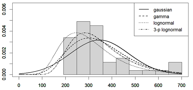
is its SD, while the index 2 refers to MAP. The correlation coefficient is unknown in this case, but I found that in a sample of 50 healthy men, its mean value is 0.3 with a 95CI between 0.1 and 0.54 (R). What we can do now for comparing the means of CP in the two populations of Table 1 is to run a Student’s t-test for any possible combination of correlation coefficients in [0.1,0.54]x[0.1,0.54], where one coefficient is for the healthy subjects, the other for the POTS group. This task is performed by the R script in the appendix (the first script). The highest p value that we obtain is about 10^{-20}, therefore the difference in CP between these two groups is exceptionally significant. Even if we run the script for correlation coefficients in [-1,1]x[-1,1] we get that the highest p value is about 2\cdot 10^{-19}. Therefore, there is no doubt that, at least for this sample and assumed true the hypotheses on the distributions of CO and MAP, the difference in CP between POTS and controls is strongly significant.

Model of cardiac power as a function of heart rate

One might expect that when there is an increase in HR, there is a reduction in SV because there is less time for the left ventricle to fill. This is, in fact, the case, and if we perform a linear regression between HR and SVI on 52 healthy subjects after 25 minutes of tilt at 70 degrees, we find

SVI\,=\,-\frac{(HR-130.7)}{1.968}

where SVI is the stroke volume normalized to body surface area (BSA) and it is expressed in \frac{ml}{m^2}. This regression is from (van Campen CLMC et al. 2023). Therefore, for CPI at the end of tilt testing, we can write

CPI\,=\,CI\times MAP\,=\,SVI\times HR\times MAP\,=\,-\frac{HR-130.7}{1.968}\times HR\times MAP

If we plot CPI as a function of HR, for three values of MAP, we have Figure 1, where CPI decreases as HR increases. Therefore, increasing HR can be considered also a strategy for maintaining MAP at a constant level, but at a lower mechanical power expenditure by the left ventricle. Note that this model has been calculated from data on healthy individuals at the end of a tilt test, and since healthy individuals do not show a substantial increase in heart rate as POTS patients do, this model might be wrong for the higher values of the abscissa.

Figure 1. CPI (watt/m^2) as a function of HR (beats/minute) for two values of MAP, for end-tilt, in healthy subjects.

Poiseuille law

According to an extremely simplified model of the circulatory system, we can use the Poiseuille law, which is the fluid dynamic equivalent of Ohm’s law. It states that CO is given by MAP divided by systemic vascular resistance (SVR). Therefore, we can write

CP\,=\,CO\times MAP\,=\,\frac{MAP^2}{SVR}

Since in POTS we can measure, at the end of the orthostatic stress, a normal MAP and an increased SVR (Stewart JM et al. 2018), it follows that there is a reduced CP.

Appendix

This is the R script that performs the Student’s t-test:

# file name: t_test_POTS
#
# Rome 1/10/2023
#
r<-seq(-0.9,0.9,by=0.1)
#
# first value is for HC, second for POTS
#
n<-c(16,32) # sample size
nA<-n[1]
nB<-n[2]
m1<-c(5.08,2.91) # mean of CO
s1<-c(0.38,0.30) # sd of CO
m2<-c(87.5,90) # mean of MAP
s2<-c(2.5,3.5) # sd of MAP
#
moments<-function(m1,m2,s1,s2,r){
  EY<-r*s1*s2+m1*m2
  VY<-(s2*m1)^2 + (s1*m2)^2 + (s1*s2)^2 + 2*r*s1*s2*m1*m2 + (r*s1*s2)^2
  SDY<-sqrt(VY)
  return(c(EY,SDY))
}
p<-matrix(nrow=length(r),ncol=length(r))
for (i in 1:length(r)) {
  for (j in 1:length(r)) {
      temp<-moments(m1[1],m2[1],s1[1],s2[1],r[i]) # controls
      mA<-temp[1]
      sA<-temp[2]
      temp<-moments(m1[2],m2[2],s1[2],s2[2],r[j]) # patients
      mB<-temp[1]
      sB<-temp[2]
      #
      sp<-sqrt(((nA-1)*sA^2 + (nB-1)*sB^2)/(nA+nB-2)) 
      TS<-abs(mA-mB)/(sp*sqrt(1/nA + 1/nB)) 
      p[i,j]<-2*pt(-TS,df=nA+nB-2,lower.tail = TRUE, log.p = FALSE)
  }
}
p_max<-max(p)

This is the Octave script that generates the plot of CPI:

% file name = CPI_POTS
% date of creation = 2/10/2023
clear all
close all
%
K=2.21*1e-06; % conversion from mmHgxml/min to watt
%
HR=[70:1:135];
MAP=[85,90,95];
for j=1:3
  for i=1:length(HR)
    CPI(j,i)=(-(HR(i)-130.7)/1.968)*HR(i)*MAP(j);
  endfor
endfor
CPI=CPI*K;
%
plot(HR,CPI(1,:),'-k','Linewidth', 1) % Healthy subjects
hold on
plot(HR,CPI(2,:),'--k','Linewidth', 1) % POTS
hold on
plot(HR,CPI(3,:),'-.k','Linewidth', 1) % POTS
legend('MAP=85 mmHg','MAP=90 mmHg','MAP=95 mmHg','location','northeast','fontsize',15)
xlabel('HR (beats/min)','fontsize',15)
ylabel('CPI (watt/m^{2})','fontsize',15)
grid on
grid minor
axis([70,130,0.1,0.5])

Probability Density of Left Ventricular Mechanical Power: derivation from metadata. Application to ME/CFS.

Probability Density of Left Ventricular Mechanical Power: derivation from metadata. Application to ME/CFS.

Studies employing tilt table testing are usually accompanied by metadata including means and standard deviations of diastolic blood pressure (DBP), systolic blood pressure (SBP), and cardiac index (CI). But the correlations between these measures are rarely shared and raw data are commonly not publicly available. Therefore, it is impossible to calculate means and standard deviations of parameters obtained by arithmetic operations from the ones mentioned, as it is the case of cardiac power index (CPI), which is given by mean arterial pressure (MAP) times CI. CPI is a measure of the mechanical power of the left ventricle, normalized to body surface area.
In this document, I propose a method for the determination of the probability density of CPI from means and standard deviations of DBP, SBP, and CI. I then apply this method to the study of CPI in myalgic encephalomyelitis/chronic fatigue syndrome (ME/CFS). I show that, according to this analysis, CPI is significantly increased in ME/CFS patients compared to controls, in a supine position, according to the metadata from a 2018 study. On the other hand, CPI is the same in the two groups, after 25-30 minutes of orthostatic stress at 70 degrees.
The method described here obtains the missing correlations by imposing that CPI displays a three-parameter lognormal distribution and that the distributions of CI, DBP, and SBP follow Gaussian laws. Several limitations of the method are discussed in the document.

***

The complete paper with all the details can be downloaded at this link as PDF. Here I show only the results on ME/CFS. I used the metadata from a 2018 paper (R) for DBP, SBP, and CI for both supine position and end-tilt (tilt table testing lasted 25-30 minutes for each participant). Measures were performed on 150 ME/CFS patients and 37 healthy controls. CI was recorded by suprasternal aortic Doppler imaging. Means and standard deviations deduced by my method for CPI in the two groups, for the two positions, are collected below. There are also two correlations: \rho_{3,4} is the Pearson correlation coefficient calculated for SBP and DBP; \rho_{1,2} is the coefficient for CI and mean arterial pressure (MAP). MAP was calculated as DBP + (SBP – DBP)/3.

The table also includes the parameters for the three-parameter lognormal densities that describe the distributions of CPI. In the following diagram, you see the densities of CPI for both ME/CFS patients and HC in a supine position.

This method presents several limitations. It is based on the assumption that the density of CPI is a three-parameter lognormal one, but this assumption was based on the study of a sample of 50 young men that I pooled from two different studies (see below). On the other hand, the ME/CFS population and the control group discussed above show a high prevalence of females. Moreover, while in the pooled sample the direct Fick method was employed for the determination of the cardiac output, this parameter was measured by echographic techniques in the ME/CFS study. It should also be noted that the Student’s t-test used for the comparison of the means might not be appropriate in the case of means from three-parameter lognormal distributions, and an ad hoc parametric test should be developed.

La Pantera

La Pantera

Traduzione della poesia omonima di Jorge Luis Borges, pubblicata la prima volta nella raccolta El oro de los tigres, nel 1972. Pur conservando il contenuto di ciascun verso, ho stravolto le parole e cambiato lo schema delle rime, isolando due quartine e due terzine.

Sull'eterna barriera la pantera 
ripeterà l'ispezione rituale 
che per sempre sarà la sua galera,
pendolo di gioia buia e letale. 
Passano mille vite oltre le sbarre
e nessuna, rimane sola e uguale
la pantera che unica può protrarre  
la rincorsa di Achille, immortale:
la distanza infinita in una cella.
Non ha mai avuto il mondo oltre la gabbia,
la carne di una tenera gazzella
che avrebbe soddisfatto la sua rabbia.
Invano offre tante strade la vita,
i suoi giorni sono grani di sabbia. 

La poesia di Borges, che si può leggere qui, pare attingere esplicitamente alla omonima lirica di Rilke del 1903, dove ritroviamo una pantera in cattività. La ispezione psicologica anche si sofferma su considerazioni analoghe. In entrambi i casi il rapporto con il mondo esterno è di completa rimozione: <<und hinter tausend Stäben keine Welt>>, nella versione icastica di Rilke; “No sabe que hay praderas y montañas\De ciervos cuyas trémulas entrañas\Deleitarían su apetito ciego“, nella interpretazione più ariosa e patetica dello scrittore argentino. Entrambi gli autori adottano poi l’idea della moltiplicazione delle barre, che il moto oscillatorio dell’animale rende infinite. Per Rilke è “Ihm ist, als ob es tausend Stäbe gäbe“; Borges invece evoca, se non mi inganna, un paradosso di Zenone, quello di Achille e della tartaruga, che per la pantera si traduce in una evasione impossibile. La corrispondenza fra la serie convergente che risolve il paradosso e la realtà cinematica della pantera non è naturalmente del tutto puntuale, perché la fiera percorre sempre lo stesso segmento, all’infinito, mentre il semidio se ne trova davanti uno via via più corto. Sarebbe più attinente la metafora del pendolo ideale, che ho provato a inserire nella mia versione. Ma ad ogni modo trovo l’immagine borgesiana una meravigliosa illuminazione. Nonostante tutto però, la poesia di Rilke sembra più efficace, almeno al mio accesso indiretto, data la mia ignoranza del tedesco; perché non necessita la protesica di questi riferimenti dotti: gode di completa autonomia. Inoltre Rilke, molto meglio di Borges, descrive la follia apatica in cui si cristallizza la volontà felina nella cattività impietosa, con una profondità ed esattezza psicologica unica forse nella letteratura. Per me, mentre Borges esegue egregiamente un esercizio poetico sulla traccia di Rilke, Rilke immortala un destino terribile e possibile, per sempre e per tutti, in una soluzione che è difficile migliorare. Nella competizione tra il vecchio poeta di Buenos Aires e il boemo neanche trentenne, per me vince il lampo di intuito giovanile.

Quella che segue è una traduzione mia dei versi di Rilke, in cui conservo lo schema delle rime e delle strofe originali. La versione mantiene l’associazione fra versi e contenuto, ma si svincola dalla completa aderenza letterale, che sarebbe del resto resa difficile dal duplice vincolo dell’endecasillabo e delle rime.

La pantera

Lo scorrere delle sbarre ha sfinito 
lo sguardo, che non trattiene più niente. 
Come se il numero fosse infinito
e oltre l'infinito, nessun presente. 

La sua andatura potente e morbida
che si volta, in quello spazio ingrato
è come danza di una forza che orbita    
attorno a un volere paralizzato.

Delle volte gli occhi seguono un'ombra
nel silenzio, che trova una via giù
nella tensione muta delle membra,
raggiunge il cuore e non esiste più.

Di seguito riporto il conteggio delle sillabe, tenendo conto delle sinalefe, e con l’indicazione degli ictus in grassetto, per la traduzione della poesia di Borges.

sul-le-ter-na-bar-rie-ra-la-pan-te-ra (11 sillabe)
ri-pe-te--li-spe-zio-ne-ri-tua-le (11 sillabe)
che-per-sem-pre-sa--la-sua-ga-le-ra (11 sillabe)
pen-do-lo-di-gio-ia-bui-ae-le-ta-le (11 sillabe)
pas-sa-no-mil-le-vi-teol-tre-le-sbar-re (11 sillabe)
e-nes-su-na-ri-ma-ne-so-laeu-gua-le (11 sillabe)
la-pan-te-ra-cheu-ni-ca-può-pro-trar-re (11 sillabe)
la-rin-cor-sa-dia-chil-le-im-mor-ta-le (11 sillabe)
la-di-stan-zain-fi-ni-tain-u-na-cel-la (11 sillabe)
non-ha-maia-vu-toil-mon-dool-tre-la-gab-bia (11 sillabe)
la-car-ne-diu-na-te-ne-ra-gaz-zel-la (11 sillabe)
chea-vreb-be-sod-di-sfat-to-la-sua-rab-bia (11 sillabe)
in-va-noof-fre-tan-te-stra-de-la-vi-ta (11 sillabe)
i-suoi-gior-ni-so-no-gra-ni-di-sab-bia (11 sillabe)

Di seguito riporto il conteggio delle sillabe, tenendo conto delle sinalefe, e con l’indicazione degli ictus in grassetto, per la traduzione della poesia di Rilke.

lo-scor-re-re-del-le-sbar-reha-sfi-ni-to (11 sillabe)
lo-sguar-do-che-non-trat-tie-ne-più-nien-te (11 sillabe)
co-me-seil-nu-me-ro-fos-sein-fi-ni-to (11 sillabe)
eol-tre-lin-fi-ni-to-nes-sun-pre-sen-te (11 sillabe)

la-su-and-a-tu-ra-po-ten-tee-mor-bi-da (12 sillabe)
che-si-vol-ta-in-quel-lo-spa-zioin-gra-to (11 sillabe)
è-co-me-dan-za-diu-na-for-za-cheor-bi-ta (12 sillabe)
at-tor-noaun-vo-le-re-pa-ra-liz-za-to (11 sillabe)

del-le-vol-te-glioc-chi-se-guo-nou-nom-bra (11 sillabe)
nel-si-len-zio-che-tro-vau-na-via-giù (10 sillabe)
nel-la-ten-sio-ne-mu-ta-del-le-mem-bra (11 sillabe)
rag-giun-geil-cuo-ree-non-e-si-ste-più (10 sillabe)

L’errore di Leopardi

L’errore di Leopardi

L’articolo può essere scaricato qui.

Giacomo Leopardi è noto soprattutto per il giardino di endecasillabi e settenari coltivato nella cornice dei primi otto lustri dell’Ottocento, l’orizzonte temporale del suo arco. Ma l’eco di quella vita, l’orma impressa dalla stampa, popola di guardie monolitiche le nostre librerie anche con una fitta prosa di trattati, tra cui una precoce ed enciclopedica Storia dell’Astronomia, di epistole, di filologia, di filosofia morale e di riflessioni tra scienze umane e naturali, ovvero i Pensieri, le Operette Morali, e le quattromila e più pagine di Zibaldone in cui tutto si embrica in un labirinto del sapere; senza contare l’affastellarsi di parole moderne da lui donate alle fatiche di Omero e di Virgilio, traducendo, entro la maggiore età, il libro primo dell’Odissea e il secondo dell’Eneide.

I Pensieri furono redatti tra il 1831 e il 1835, per lo più a Napoli, sotto le premure di Paolina, sorella acquisita per la proprietà transiva dell’affetto; in maggior parte sintesi delle scintille di etologia umana dello Zibaldone. Ma mai conclusi davvero dal poeta, furono finiti dalla sua fine, e poi fatti conoscere da una stampa postuma per i tipi di Le Monnier e per la volontà di Ranieri, nel 1845. Un catalogo di centoundici appunti di viaggio sui primati bipedi, ironici e amari, misogini e disincantati. Machiavellismo sociale, secondo una definizione dell’autore.

Nel ventesimo pensiero Leopardi ventila la possibilità di speculare, nel mondo parallelo dei paradossi, sulla pandemica diffusione del vizio degli uomini di scrivere e di voler leggere i propri ingegni letterari agli amici; propone che si istituisca “una scuola o accademia ovvero ateneo di ascoltazione; dove, a qualunque ora del giorno e della notte, essi, o persone stipendiate da loro, ascolteranno chi vorrà leggere a prezzi determinati: che saranno per la prosa, la prima ora, uno scudo, la seconda due, la terza quattro, la quarta otto, e così crescendo con progressione aritmetica. Per la poesia il doppio.

E’ prezioso qui il riferimento alla progressione aritmetica, ma è sbagliato. Infatti, una successione di termini a_1 ,\,a_2 ,\,... si chiama progressione aritmetica quando, comunque si scelga n\,>\,2, si ha:

a_n\,-a_{n-1}\,=\,r_{a}

dove r_{a} assume il nome di ragione aritmetica. Altresì, una successione si dice geometrica quando

\frac{a_n}{a_{n-1}}\,=\,r_{g}

In questo caso si parla per r_{g} di ragione geometrica. E dunque la menzionata successione di esborsi con cui tassare gli autori molesti è una progressione geometrica, non aritmetica.

Può tuttavia sorgere il dubbio che in passato le due successioni rispondessero ad altri nomi. A tal proposito, abbiamo conoscenza dei manuali di matematica presenti nella celebrata libreria del conte Monaldo Leopardi, padre di Giacomo; tra essi gli Elementi di Matematica di Vito Caravelli (1770) [1]. E andando a recuperare il testo, scopriamo che le definizioni di progressione aritmetica e geometrica si trovano nei capitoli III (pagina 253) e IV (pagina 258), rispettivamente, di suddetto libro. Le due pagine menzionate sono riportate in figura e, come si può leggere, le definizioni date coincidono con quelle oggi in uso. Si noti tra l’altro che l’esempio di progressione geometrica crescente portato da Caravelli coincide con la successione usata da Leopardi nel suo testo, nutrendo almeno la suggestione che in effetti l’autore ricordasse proprio questa fonte.

Mi sono chiesto allora, proprio principiando dalla pagina dei Pensieri, quale fosse il rapporto di Leopradi con la matematica e ho interrogato per questo lo Zibaldone. Se si naviga il testo con la chiave “progressione” ci si imbatte in un riferimento del 1821 alla progressione geometrica. Ci troviamo a pagina 1924 del testo autografo:

<<L’andamento, o il così detto perfezionamento dello spirito umano rassomiglia interamente alla progressione geometrica che dal menomo termine, con proporzione crescente arriva all’infinito>>.

E alcune righe sotto, ad inizio della pagina seguente, in una variante per lo più tautologica e permutativa, leggiamo:

<<E non è dubbio che quella che si chiama perfettibilità dell’uomo è suscettibile di aumento in infinito come la progressione geometrica, e di un aumento sempre proporzionalmente maggiore>>.

Mi sembra che anche mettendo insieme le due proposizioni, non si pervenga con sicurezza a una definizione della progressione geometrica, come se l’autore non avesse in mente un riferimento puntuale ad essa ma ne usasse il nome per il suo valore evocativo.

Se si interroga lo Zibaldone con la parola “matematica”, si trova, a pagina 46 del manoscritto autografo, il seguente sillogismo, mutilato della conclusione:

<<La grazia non può venire altro che dalla natura, e la natura non istà mai secondo il compasso della gramatica della geometria dell’analisi della matematica ec.>>.

Siamo tra il 1818 e il 1820 e il giovane Leopardi sembra affermare che la natura non può essere descritta dalla matematica, una delle due premesse, e che la grazia non può attingere alla matematica, conclusione questa che potrei però avere frainteso. La premessa menzionata è ribadita altrove, già solo fermanadosi alle prime seicento pagine del testo. A pagina 583, siamo nel 1821, si legge:

<<E dovunque ha luogo la perfezione matematica, ha luogo una vera imperfezione (quando anche questa rimedii ad altri più gravi inconvenienti e corruzioni), cioè discordanza dalla natura, e dall’ordine primitivo delle cose, il quale era combinato in altro modo, e fuor del quale non v’è perfezione, benchè questa non sia mai assoluta, ma relativa>>.

A cavallo tra le pagine 584 e 585, Leopardi ribadisce:

<<Questa pure è una gran fonte di errori ne’ filosofi, massime moderni, i quali assuefatti all’esattezza e precisione matematica, tanto usuale e di moda oggidì, considerano e misurano la natura con queste norme, credono che il sistema della natura debba corrispondere a questi principii; e non credono naturale quello che non è preciso e matematicamente esatto: quando anzi per lo contrario, si può dir tutto il preciso non è naturale: certo è un gran carattere del naturale il non esser preciso>>.

Sembra certo allora che Leopardi sia convinto che la matematica non sia lo strumento adatto a descrivere la natura, posizione che lo vede solitario, consapevole di esserlo. E non sembrano esserci dubbi sulla accezione da selezionare per “natura”, perché proprio il poeta ce l’ha presentata questa accezione, letteralmente, nella sua letteratura: ha dialogato con essa, travestito da islandese, da qualche parte, in Africa, vicino l’equatore.

E dunque, se non ho frainteso tutto, Leopardi tradisce Galileo e Newton, di cui tuttavia menziona correttamente – sebbene in modo qualitativo – i risultati già nella citata storia dell’astronomia, scritta a quindici anni; quel monumento di oltre 400 pagine popolate da citazioni in varie lingue, sia parlate che seppellite, e scoperte che partendo dagli astronomi Caldei, arrivano all’anno 1813. Il ragazzo che fu menzionava diligentemente la legge di caduta dei gravi, a velocità linearmente crescente con il tempo, le leggi di Keplero, alcuni dei risultati di Newton. Ma è come se non avesse inteso la lezione principale del diciassettesimo secolo, quella che denuncia tutta l’opera, non solo dei due grandi, ma di Torricelli, Cavalieri, Stevin, Pascal, e altri, e che trova l’enunciato più esplicito e noto nel Galileo del Saggiatore, che dice:

<<La filosofia naturale è scritta in questo grandissimo libro che continuamente ci sta aperto innanzi agli occhi, io dico l’universo, ma non si può intendere se prima non s’impara a intender la lingua e conoscer i caratteri nei quali è scritto. Egli è scritto in lingua matematica, e i caratteri son triangoli, cerchi ed altre figure geometriche, senza i quali mezzi è impossibile a intenderne umanamente parola; senza questi è un aggirarsi vanamente per un oscuro labirinto>>.

Senza contare che Leopardi nasce dopo tutta la vita di Eulero, è contemporaneo di Fourier e di Gauss, è di sessant’anni più giovane di Lagrange. Ovvero vive l’epopea del calcolo differenziale come impareggiabile chiave decifrativa di ogni aspetto della natura, e sembra non accorgersene.

Resta il punto sulla grazia e la matematica. A cavallo tra pagina 247 e 248, nel 1820, l’autore scrive:

<<Perciò la matematica la quale misura quando il piacer nostro non vuol misura, definisce e circoscrive quando il piacer nostro non vuol confini (sieno pure vastissimi, anzi sia pur vinta l’immaginazione dalla verità), analizza, quando il piacer nostro non vuole analisi nè cognizione intima ed esatta della cosa piacevole (quando anche questa cognizione non riveli nessun difetto nella cosa, anzi ce la faccia giudicare più perfetta di quello che credevamo, come accade nell’esame delle opere di genio, che scoprendo tutte le bellezze, le fa sparire), la matematica, dico, dev’esser necessariamente l’opposto del piacere>>.

La matematica dunque è contraria al piacere e sottrae la bellezza a ciò che è bello. Una posizione questa difficilmente condivisibile, quanto largamente condivisa; per restare negli stessi anni, ma cambiando lato dello iato oceanico, Edgar Allan Poe si esprimeva in modo analogo nei confronti della scienza [2]:

Science! true daugther of Old Time thou art!
Who alterest all things with thy peering eyes.
Why preyest thou upon the poet's heart,
Vulture, whose wings are dull realities?

Ma volendo anche in questo caso risolvere la questione con parole altrui, interpello Godfred Harold Hardy:

<<The mathematician’s patterns, like the painter’s or the poet’s, must be beautiful; the ideas, like the colours or the words, must fit together in a harmonious way. Beauty is the first test: there is no permanent place in the world for ugly mathematics>>.

E inoltre:

<<It would be difficult now to find an educated man quite insensitive to the aesthetic appeal of mathematics>> [3].

Cosa si trova se si invoca ancora lo Zibaldone in nome di Galileo? C’è una osservazione di pagina 2013 (autunno del 1821), fra le altre, che lo menziona in rapporto a quanto espresso sulla matematica:

<<Torno a dire che la precisione moderna ch’è estrema, e che in tali scritti e generi è di prima necessità, e che oggi si ricerca sopra tutte le qualità ec. è assolutamente di sua natura incompatibile colla eleganza: ed infatti il nostro secolo che è quello della precisione, non è certo quello della eleganza in nessun genere. Bensì ell’è compatibilissima colla purità, come si può vedere in Galileo, che dovunque è preciso e matematico quivi non è mai elegante, ma sempre purissimo italiano>>.

Cioè Leopardi afferma che dove Galileo usa un linguaggio matematico non può essere elegante, coerentemente con quanto enunciato sulla matematica. Perché per Leopardi, come sappiamo, l’eleganza è appannaggio dell’indefinito:

<<Se attentamente riguarderemo in che soglia consistere l’eleganza delle parole, dei modi, delle forme, dello stile, vedremo quanto sovente anzi sempre ella consista nell’indeterminato, (v. in tal proposito quello che altrove ho detto circa un passo di Orazio) v. p.1337. principio o in qualcosa d’irregolare, cioè nelle qualità contrarie a quelle che principalmente si ricercano nello scrivere didascalico o dottrinale. Non nego io già che questo non sia pur suscettibile di eleganza, massime in quelle parti dove l’eleganza non fa danno alla precisione, vale a dire massimamente nei modi e nelle forme. E di questa associazione della precisione coll’eleganza, è splendido esempio lo stile di Celso, e fra’ nostri, di Galileo>>.

Quindi, nonstante la tensione verso la precisione che inaridisce, Leopardi non riesce a negare di ammirare la prosa di Galileo. E Galilei, tra le osservazioni sperimentali e le argomentazioni geometriche che hanno cambiato il mondo e fatto tremare gli dèi, ha effettivamente seminato dei paragrafi che rappresentano forse la migliore letteratura italiana:

<<Né sia chi creda che la lettura de gli altissimi concetti, che sono scritti in quelle carte, finisca nel solo vedere lo splendore del Sole e delle stelle e ‘l lor nascere ed ascondersi, che è il termine sin dove penetrano gli occhi dei bruti e del vulgo; ma vi son dentro misteri tanto profondi e concetti tanto sublimi, che le vigilie, le fatiche e gli studi di cento e cento acutissimi ingegni non gli hanno ancora interamente penetrati con l’investigazione continuate per migliaia e migliaia d’anni. E credino pure gli idioti che, sì come quello che gli occhi loro comprendono nel riguardo l’aspetto esterno d’un corpo umano è piccolissima cosa in comparazione de gli ammirandi artifizi che in esso ritrova un esquisito e diligentissimo anatomista e filosofo, mentre va investigando l’uso di tanti muscoli, tendini, nervi ed ossi, essaminando gli offizi del cuore e de gli altri membri principali, ricercando le sedi delle facoltà vitali, osservando le meravigliose strutture de gli strumenti de’ sensi, e, senza finir mai di stupirsi e di appagarsi, contemplando i ricetti dell’immaginazione, della memoria e del discorso; così quello che ‘l puro senso della vista rappresenta, è come nulla in proporzion dell’alte meraviglie che, mercè le lunghe ed accurate osservazioni, l’ingegno degli intelligenti scorge nel cielo>> [4].

Una possibile conclusione di questa breve esplorazione è che Leopardi sia stato vittima di una educazione incompleta; incredibilmente, vista la dimensione borgesiana della biblioteca paterna, che includeva anche le opere originali di Galileo e Newton. E’ stato in effetti suggerito che il recanatese non conobbe mai i logaritmi, introdotti già da quasi duecento anni, e non avesse studiato né la geometria analitica di Descartes, né il calcolo differenziale, che pure era vecchio di almeno un secolo alla sua nascita [1]. Può darsi che il poeta abbia ereditato un peccato paterno: se si confronta il piano di studi dell’educazione domestica matematica di Leopardi con il tipo di istruzione impartita nelle università spagnole del diciottesimo secolo, si trova una sovrapponibilità [1], [5]. Se chiedo al lettore il nome di un matematico spagnolo dell’epoca di Galilei e dei due secoli successivi, cosa mi dice? Esatto! Il calcolo differenziale arrivò in Spagna, in una forma didattica e non investigativa, solo dopo la cacciata dell’ordine dei Gesuiti (1767), con il ricambio del corpo docente. Fino ad allora, la matematica rimase cristallizzata nelle formule algebriche e nei teoremi di Euclide, umiliate spesso dalle semplici applicazioni finanziarie, di agronomia, e militari. E dopo progredì solo come un corpo minato da una grave malattia [5]. E dove apprese Monaldo la sua scienza? Il suo precettore fu un Giuseppe Torres, gesuita approdato in Italia dal rifiuto spagnolo del suo ordine. E’ possibile che la nuova matematica fosse troppo indissolubilmente legata alla nuova fisica, per questo condannata ad essere rifiutata con essa dai monopolisti gesuiti del sapere. Con il risultato che la storia della matematica moderna sarebbe forse la stessa se la Spagna non fosse mai esistita.

L’errore di Leopardi non sarebbe dunque quello della confusione tra la progressione aritmetica e quella geometrica, che non ha nessuna importanza, ma quello di essersi fermato sulla soglia di un mondo che forse avrebbe potuto soddisfare il suo anelito alla bellezza e alla felicità. Si affrancò dal sistema tolemaico, ma non dalla ignoranza che lo sottendeva. E ora che scrivo, aggiungendo una pagina al mio modesto Zibaldone, e me lo figuro ragazzo nelle ore dilatate dalla giovinezza, in quella dimora privilegiata che gli fu così angusta, mi piace immaginarlo distratto, su quella soglia, dal fascino opalino della Luna, o dal fruscio delle vesti di una Nerina di cui è stato da tempo dimenticato il nome.

Riferimenti

[1] M.T. Borgato, L. Pepe, Leopardi e le Scienze Matematiche, 1998

[2] E.A. Poe, Sonnet – To Science, vv 1-4, scritto e rimaneggiato tra il 1829 e il 1845

[3] G.H. Hardy, A Mathematician’s Apology, 1940

[4] G. Galilei, Lettera a Cristina di Lorena, 1615

[5] C. López-Esteban, A. Maz-Machado, Las matemáticas en España durante el siglo XVIII a través de los libros y sus autores, 2020

Il testo completo dei Pensieri si può consultare qui. Una edizione di questa opera con i commenti di Paolo Emilio Castagnola è disponibile qui. La edizione del 1770 degli Elementi di Matematica di Vito Caravelli è disponibile qui. Una copia completa dello Zibaldone può essere scaricata in pdf qui. Nel film su Leopardi di Mario Martone del 2014, Il giovane favoloso, la sezione del pensiero XX qui discussa è messa in bocca allo stesso poeta, durante una cena romana, presso dei parenti, e la menzione alla progressione aritmetica è stata eliminata, probabilmente perché ci si è resi conto della svista del poeta, e non potendo modificare le sue parole, le si è tagliate.

Human proportions

Human proportions

Artists have proposed different proportions for the human body, throughout history. In ancient Egypt, the height of a human figure was set at 6.33 times the length of his foot [1]. For Michelangelo, as well as for Lisippo, the ideal height of a man was 8 times the head [1], [2]. In 1958, Burne Hogarth proposed as a reference for human proportions an imposing frame standing more than 190 cm tall, about 8.7 times the head [3].

But what do we know about human proportions, from an experimental point of view? I considered a 1972 paper by Renato Contini (destined for laboratories that manufacture prosthetic limbs) with several geometric and mechanic measures on the bodies of a group of US citizens, both males and females. In particular, I considered the measures reported in Figures 7 and 8 of the aforementioned paper [4], where the length of the segments of the body is expressed as a function of the height, H. The problem with the illustrations in the original paper is that they do not respect the proportions reported on the figures themselves (figure 1). Therefore, they are pretty confusing for the artist.

Figure 1. The original illustration of [4]. I used the proportions that refer to the US population. H: total height.

In order to generate an illustration that faithfully represented the proportions experimentally determined by Contini, I wrote an Octave script (reported at the end of this article) which generates Figure 2, where the proportions are indicated in a way that is probably more useful for the artist: I express the lengths of the limbs as a function of both H and of h. This same script can be used to compare a male and a female of the same height (figure 3). The female body is exactly 8 times the head, while the male body is only 7.69 times the head. The head of a male is bigger than the head of a female of the same height, the shoulders are wider, and the hips are tighter, as expected. The relative length of the torso is a bit longer in women than in men. A woman stands 6.62 times her foot, a man 6.58; therefore the Egyptian statues had longer feet, in proportion, than the average US citizen.

Figure 2. The proportions of the human body, according to Contini [4]. I considered a female of 161.3 cm (left) and a male of 175.3 cm (right). H: total height; h: head.

Figure 3. The proportions of the human body, according to Contini [4]. I considered a female (left) and a male (right) of the same height (170.0 cm). H: total height; h: head.

References

[1] De Simoni Luigi, De Simoni Piero, Anatomia Umana Artistica, Volume I, Bonacci Editore, Roma 1986

[2] Bridgman George B, Bridgman’s Life Drawing, Dover Publications, New York, 1924

[3] Hogarth Burne, Dynamic Anatomy, Watson-Guptill Publications, New York, 1958

[4] Contini Renato, Body Segment Parameters, Part II, 1972

The script

% file name = Contini
% date of creation = 23/05/2023
%
close all
clear all
%
%-------------------------------------------------------------------------------
% US population
%-------------------------------------------------------------------------------
%
height(1) = 161.3; % height of female (cm)
height(2) = 175.3; % height of male (cm)
width1 = [0.245*height(1),0.259*height(2)]; % from the tip of one clavicole to the tip of the other
width2 = [0.219*height(1),0.200*height(2)]; % from one head of one femur to the head of the other
width3 = [0.057*height(1),0.055*height(2)]; % width of the footh
Length1 = [0.938*height(1),0.936*height(2)];
Length2 = [0.875*height(1),0.870*height(2)];
Length3 = [0.825*height(1),0.819*height(2)];
Length4 = [0.632*height(1),0.630*height(2)];
Length5 = [0.480*height(1),0.485*height(2)];
Length6 = [0.370*height(1),0.357*height(2)];
Length7 = [0.524*height(1),0.530*height(2)];
Length8 = [0.282*height(1),0.285*height(2)];
Length9 = [0.048*height(1),0.043*height(2)];
js = 5 % joint size
shift = [0,100] % I use this to shift the second plot on the right
%
figure(1)
%
for (i=1:2)
  %
  H = height(i)
  w1 = width1(i)
  w2 = width2(i)
  w3 = width3(i)
  L1 = Length1(i)
  L2 = Length2(i)
  L3 = Length3(i)
  L4 = Length4(i)
  L5 = Length5(i)
  L6 = Length6(i)
  L7 = Length7(i)
  L8 = Length8(i)
  L9 = Length9(i)
  h = H - L2 % head height
  l = h/3 % head width divided by two
  %
  %-------------------------------------------------------------------------------
  % bones
  %-------------------------------------------------------------------------------
  %
  plot([0+shift(i),0+shift(i)],[H-h,L7],"-k","linewidth",1.5) % backbone
  hold on
  rectangle ("Position",[-l+shift(i),H-h,2*l,h],"linewidth",1.5) % head
  plot([-l+shift(i),l+shift(i)],[L1,L1],"-k","linewidth",1.5) % eyes
  %
  plot([-w1/2+shift(i),w1/2+shift(i)],[L3,L3],"-k","linewidth",1.5) % shoulders (tips of the clavicles)
  %
  plot([-w1/2+shift(i),-w1/2+shift(i)],[L3,L4],"-k","linewidth",1.5) % homerus, left
  plot([w1/2+shift(i),w1/2+shift(i)],[L3,L4],"-k","linewidth",1.5) % homerus, rigth
  %
  plot([-w1/2+shift(i),-w1/2+shift(i)],[L4,L5],"-k","linewidth",1.5) % radius, left
  plot([w1/2+shift(i),w1/2+shift(i)],[L4,L5],"-k","linewidth",1.5) % radius, rigth
  %
  rectangle ("Position",[-w1/2-(3/4)*l/2+shift(i),L6,(3/4)*l,L5-L6],"linewidth",1.5) % hand, left
  rectangle ("Position",[w1/2-(3/4)*l/2+shift(i),L6,(3/4)*l,L5-L6],"linewidth",1.5) % hand, rigth
  %
  plot([-w2/2+shift(i),w2/2+shift(i)],[L7,L7],"-k","linewidth",1.5) % hip
  %
  plot([-w3+shift(i),w3+shift(i)],[0,0],"-k","linewidth",1.5) % feet, plant
  %
  plot([-w3+shift(i),-w3/2+shift(i)],[0,L9],"-k","linewidth",1.5) % ankle, left
  plot([-w3/2+shift(i),0+shift(i)],[L9,0],"-k","linewidth",1.5) % ankle, left
  plot([0+shift(i),w3/2+shift(i)],[0,L9],"-k","linewidth",1.5) % ankle, rigth
  plot([w3/2+shift(i),w3+shift(i)],[L9,0],"-k","linewidth",1.5) % ankle, rigth
  %
  plot([-w3/2+shift(i),-w3+shift(i)],[L9,L8],"-k","linewidth",1.5) % tibia, left
  plot([w3/2+shift(i),w3+shift(i)],[L9,L8],"-k","linewidth",1.5) % tibia, rigth
  %
  plot([-w2/2+shift(i),-w3+shift(i)],[L7,L8],"-k","linewidth",1.5) % femur, left
  plot([w2/2+shift(i),w3+shift(i)],[L7,L8],"-k","linewidth",1.5) % femur, rigth
  %
  %-------------------------------------------------------------------------------
  % joints
  %-------------------------------------------------------------------------------
  %
  plot(-w1/2+shift(i),L3,'o','markersize',js,'markerfacecolor','k','markeredgecolor','k') % shoulder, left
  plot(w1/2+shift(i),L3,'o','markersize',js,'markerfacecolor','k','markeredgecolor','k') % shoulder, rigth
  %
  plot(-w1/2+shift(i),L4,'o','markersize',js,'markerfacecolor','k','markeredgecolor','k') % elbow, left
  plot(w1/2+shift(i),L4,'o','markersize',js,'markerfacecolor','k','markeredgecolor','k') % elbow, rigth
  %
  plot(-w1/2+shift(i),L5,'o','markersize',js,'markerfacecolor','k','markeredgecolor','k') % wirst, left
  plot(w1/2+shift(i),L5,'o','markersize',js,'markerfacecolor','k','markeredgecolor','k') % wirst, rigth
  %
  plot(-w2/2+shift(i),L7,'o','markersize',js,'markerfacecolor','k','markeredgecolor','k') % hip, left
  plot(w2/2+shift(i),L7,'o','markersize',js,'markerfacecolor','k','markeredgecolor','k') % hip, rigth
  %
  plot(-w3+shift(i),L8,'o','markersize',js,'markerfacecolor','k','markeredgecolor','k') % knee, left
  plot(w3+shift(i),L8,'o','markersize',js,'markerfacecolor','k','markeredgecolor','k') % knee, rigth
  %
  plot(-w3/2+shift(i),L9,'o','markersize',js,'markerfacecolor','k','markeredgecolor','k') % ankle, left
  plot(w3/2+shift(i),L9,'o','markersize',js,'markerfacecolor','k','markeredgecolor','k') % ankle, rigth
  %
  %-------------------------------------------------------------------------------
  % measures
  %-------------------------------------------------------------------------------
  %
  L = H/3;
  % head
  plot([-L+shift(i),0+shift(i)],[H,H],"--k","linewidth",1.0)
  plot([-L+shift(i),0+shift(i)],[H-h,H-h],"--k","linewidth",1.0)
  quiver(-L+shift(i),H-h,0,h,'-k',"maxheadsize",0.1)
  quiver(-L+shift(i),H,0,-h,'-k',"maxheadsize",0.1)
  factorH = h/H;
  text (-L+l/2+shift(i),H-h/2,strcat("h=",num2str(factorH),"H"),"fontsize",15)
  % homer
  homer = L3 - L4;
  plot([-L+shift(i),-w1/2+shift(i)],[L3,L3],"--k","linewidth",1.0)
  plot([-L+shift(i),-w1/2+shift(i)],[L4,L4],"--k","linewidth",1.0)
  quiver(-L+shift(i),L4,0,homer,'-k',"maxheadsize",0.1)
  quiver(-L+shift(i),L3,0,-homer,'-k',"maxheadsize",0.1)
  factorH = homer/H;
  factorh = homer/h;
  text (-L+l/2+shift(i),L3-homer/2,strcat(num2str(factorH),"H=",strcat(num2str(factorh),"h")),"fontsize",15)
  % radius
  radius = L4 - L5;
  plot([-L+shift(i),-w1/2+shift(i)],[L4,L4],"--k","linewidth",1.0)
  plot([-L+shift(i),-w1/2+shift(i)],[L5,L5],"--k","linewidth",1.0)
  quiver(-L+shift(i),L5,0,radius,'-k',"maxheadsize",0.1)
  quiver(-L+shift(i),L4,0,-radius,'-k',"maxheadsize",0.1)
  factorH = radius/H;
  factorh = radius/h;
  text (-L+l/2+shift(i),L4-radius/2,strcat(num2str(factorH),"H=",strcat(num2str(factorh),"h")),"fontsize",15)
  % hand
  hand = L5 - L6;
  plot([-L+shift(i),-w1/2+shift(i)],[L5,L5],"--k","linewidth",1.0)
  plot([-L+shift(i),-w1/2+shift(i)],[L6,L6],"--k","linewidth",1.0)
  quiver(-L+shift(i),L6,0,hand,'-k',"maxheadsize",0.1)
  quiver(-L+shift(i),L5,0,-hand,'-k',"maxheadsize",0.1)
  factorH = hand/H;
  factorh = hand/h;
  text (-L+l/2+shift(i),L5-hand/2,strcat(num2str(factorH),"H=",strcat(num2str(factorh),"h")),"fontsize",15)
  % femur
  femur = L7 - L8;
  plot([-1.1*L+shift(i),-w1/2+shift(i)],[L7,L7],"--k","linewidth",1.0)
  plot([-1.1*L+shift(i),-w3+shift(i)],[L8,L8],"--k","linewidth",1.0)
  quiver(-1.1*L+shift(i),L8,0,femur,'-k',"maxheadsize",0.1)
  quiver(-1.1*L+shift(i),L7,0,-femur,'-k',"maxheadsize",0.1)
  factorH = femur/H;
  factorh = femur/h;
  text (-1.1*L+l/2+shift(i),L7-homer,strcat(num2str(factorH),"H=",strcat(num2str(factorh),"h")),"fontsize",15)
  % tibia
  tibia = L8 - L9;
  plot([-L+shift(i),-w3+shift(i)],[L8,L8],"--k","linewidth",1.0)
  plot([-L+shift(i),-w3/2+shift(i)],[L9,L9],"--k","linewidth",1.0)
  quiver(-L+shift(i),L8,0,-tibia,'-k',"maxheadsize",0.1)
  quiver(-L+shift(i),L9,0,tibia,'-k',"maxheadsize",0.1)
  factorH = tibia/H;
  factorh = tibia/h;
  text (-L+l/2+shift(i),L8-tibia/2,strcat(num2str(factorH),"H=",strcat(num2str(factorh),"h")),"fontsize",15)
  % ankle
  ankle = L9;
  plot([-L+shift(i),-w3/2+shift(i)],[0,0],"--k","linewidth",1.0)
  quiver(-L+shift(i),L9,0,-ankle,'-k',"maxheadsize",0.1)
  quiver(-L+shift(i),0,0,ankle,'-k',"maxheadsize",0.1)
  factorH = ankle/H;
  factorh = ankle/h;
  text (-L+l/2+shift(i),L9-ankle/2,strcat(num2str(factorH),"H=",strcat(num2str(factorh),"h")),"fontsize",15)
  % shoulders
  quiver(-w1/2+shift(i),L3-l,w1/2,0,'-k',"maxheadsize",0.1)
  quiver(0+shift(i),L3-l,-w1/2,0,'-k',"maxheadsize",0.1)
  factorH = w1/(2*H);
  factorh = w1/(2*h);
  text (-2*l+shift(i),L3-2*l,strcat(num2str(factorH),"H=",strcat(num2str(factorh),"h")),"fontsize",15,"backgroundcolor","white")
  % hips
  plot([-w2/2+shift(i),-w2/2+shift(i)],[L7,L7+2*l],"--k","linewidth",1.0)
  quiver(-w2/2+shift(i),L4-l,w2/2,0,'-k',"maxheadsize",0.1)
  quiver(0+shift(i),L4-l,-w2/2,0,'-k',"maxheadsize",0.1)
  factorH = w2/(2*H);
  factorh = w2/(2*h);
  text (-2*l+shift(i),L4-1.7*l,strcat(num2str(factorH),"H=",strcat(num2str(factorh),"h")),"fontsize",15,"backgroundcolor","white")
  % heads
  plot([w2/2+1.5*l+shift(i),w2/2+1.5*l+shift(i)],[H,0],"-k","linewidth",1.0)
  temp=0;
  while (temp<=H)
    plot(w2/2+1.5*l+shift(i),H-temp,'^','markersize',js,'markerfacecolor','k','markeredgecolor','k')
    temp=temp+h;
  endwhile
endfor
%
%-------------------------------------------------------------------------------
% grid and axes
%-------------------------------------------------------------------------------
%
axis([-70,140,-l,H+l],"equal")
ylabel("cm","fontsize",15)
grid on
grid minor

Non Solo Fatica, il mio intervento

Il mio intervento durante il convegno online Non Solo Fatica (15 aprile 2023). Riporto i risultati di una serie di analisi statistiche sui dati genetici di 1659 pazienti con ME/CFS. Le slide dell’intervento possono essere scaricate qui. L’intero convegno può essere visto gratuitamente a questo indirizzo, previa iscrizione.

The measure of Dante’s Universe

The measure of Dante’s Universe

At the end of the twenty-seventh canto of Paradiso (Divine Comedy), Dante Alighieri describes his ascension towards the ninth sphere of the Ptolemaic model of the universe: the Primum Movens, which contains and gives motion to all the previous skies (Moon, Mercury, Venus, Sun, Mars, Jupiter, Saturn, and Fixed Stars), that rotate around the center of the Universe, the Earth (Figure 1, left). Beatrice, the woman who leads the poet in his itinerarium in deum, explains that the Universe has a fixed center, the Earth, surrounded by eight rotating spheres or skies with an increasing radius, and all these physical elements are included in a ninth sphere, the Primum Movens, from which the movement arises; and this last sphere is not contained by other skies and has no physical place: it exists in the mind of God. The following are the verses in which Beatrice explains the mentioned architecture of the Ptolemaic system.

Ma ella che vedea il mio disire,
incominciò, ridendo tanto lieta, 
che Dio parea nel suo volto gioire:
"La natura del mondo, che quieta
il mezzo e tutto l'altro intorno move,
quinci comincia come da sua meta.
E questo cielo non ha altro dove
che la mente divina, in che s'accende
l'amor che 'l volge e la virtù ch'ei piove.
Luce ed amor d'un cerchio lui comprende
si come questo li altri; e quel precinto
colui che 'l cinge solamente intende."

Paradiso, XXVII, vv 103-114

At the beginning of canto XXVIII, Dante can now see what is beyond the Primum Movens, a reality called Empyreal, which has a structure that is symmetric to the one of the Ptolemaic universe, but this time God is the center and nine spheres or skies rotate around him (Figure 1, right; Figure 2). The union of these two points, the Erath and God, and of the two sets of nine spheres that include them, is the complete sum of all that exists, according to Dante: of what has been created and of its Creator. But what is its shape or geometric nature? If we imagine Dante as a bi-dimensional being and if we subtract a spatial dimension from all his surroundings, we can see the spheres as circles and assemble them as the parallels of a sphere of which the Earth is one pole and God is the other. Dante moves on the surface of this sphere (a space with two dimensions) and the circles are the intersection of the sphere itself with a family of parallel planes. If we now add again the third dimension to this model, we must conclude that the universe is a four-dimensional sphere and that the skies are its intersections with a family of three-dimensional spaces.

Figure 1. The Ptolemaic system, on the left. On the right, the structure of the Empyreal. From the paper by Peterson mentioned in below.

I found the idea of the universe of Dante as a hypersphere of a space with four dimensions in a 1979 paper by the physicist Mark A. Peterson, “Dante and the 3-sphere” (link). That said, it is possible to calculate the space (in four dimensions) occupied by such a universe. If we introduce a Euclidean space of dimension 4, we can calculate the volume of the sphere of radius R and center in the origin of the coordinate system, by solving the integral:

V(4,R)=2^4\int_{0}^{R}\int_{0}^{\sqrt{R^2-x_4^2}}\int_{0}^{\sqrt{R^2-\left(x_3^2+x_4^2\right)}}\int_{0}^{\sqrt{R^2-\left(x_2^2+x_3^2+x_4^2\right)}}dx_1dx_2dx_3dx_4

With a few passages, we get

V(4,R)=4\pi\left(\pi\frac{R^4}{4}-\frac{1}{3}\int_{0}^{R}\left(R^2-x_4^2\right)^\frac{3}{2}dx_4-\int_{0}^{R}x_4^2 \sqrt{R^2-x_4^2}dx_4\right)

The two integrals inside the brackets can be easily solved by integration by series (use the binomial expansion) and we get that

V(4,R)= \frac{\pi^2}{2}R^4

What is the value of R? It should be the radius of the largest sphere, the equatorial one: the Primum Movens. But it has no radius, to my knowledge, it is not material. We can use the radius of the sphere of the fixed stars, though, that according to Ptolemy (Almagest, book I, chapter V) is about 20 thousand times the radius of the Earth, r_T = 6,371 km . Therefore, we conclude that the volume of the four-dimensional hypersphere that includes the Universe, according to Dante Alighieri, is 8\pi^210^{16}r_T^4, which is about 1.3\cdot10^{45}m^4 . It is not clear what the meaning of this analysis might be, if any: Dante did not know geometry with more than three dimensions, to my knowledge. But one implication is that a three-dimensional being can not move from one sky of the Ptolemaic system to the other (because they are in different three-dimensional spaces) unless he finds a way to move along the fourth dimension. I think that this would resonate with Dante’s mind and that this would agree with what he had envisioned: he can accomplish his ascent to God only because of external intervention and help from Beatrice.

Figure 2. Dante and Beatrice in the Empyreal, incision by Gustave Doré.

Myalgic Encephalomyelitis Chronic Fatigue at the National Institutes of Health

Myalgic Encephalomyelitis Chronic Fatigue at the National Institutes of Health

Introduction

I summarize in Table 1 the results of a single-center, exploratory, cross-sectional study of post-infectious Myalgic Encephalomyelitis (PI-ME/CFS) conducted by the National Institute of Health, from October 2016 to January 2022. All the details of the study are available at this address. I run, for each measure, a statistical test. The analysis was performed by a custom R script (see the last paragraph).

Results

After correction for multiple comparisons, the only statistically significant difference between patients and controls is the number of bacterial species in the stool sample, which is lower in patients than in healthy controls (LTK, measure 11). If we do not consider the correction for multiple comparisons, we find also a lower oxygen consumption at the anaerobic threshold during the cardiopulmonary exercise test (ATVO2rel, measure 1) and a reduced variability in heart rate over a 24-hour period (SDNNi, measure 9). Perhaps surprisingly, both the total power consumed by the individuals as measured by a metabolic chamber (TBEU, 3) and the oxygen consumption of peripheral blood mononuclear cells per unit of time (MEFA, 8), are the same in patients and controls.

Table 1. For the meaning of the labels in the Test column, see below. The second column is the number associated with the test on the Results page (here). Healthy controls are indicated with the letter A, ME/CFS patients with B. The number of participants is labeled with the letter n. The means are marked with the letter m and the standard errors with the letter s. The p values are calculated with the double-tailed Student’s T-test and the corrected p values (last column) are computed employing the Benjamini-Hochberg correction.

ATVO2rel [1]. The Relative Volume of Oxygen at the Anaerobic Threshold (ATVO2rel) was determined during a cardiopulmonary exercise test (CPET). ATVO2rel represents the volume of oxygen consumed when a participant reaches AT, adjusted for their weight during the CPET. Results compared Healthy Volunteer Participants to ME/CFS Participants. Unit of Measure: mL/kg/min.

RER [2]. The Respiratory Exchange Ratio (VCO2/VO2) was determined during a cardiopulmonary exercise test (CPET). VCO2/VO2 is calculated by measuring the volume of carbon dioxide and oxygen the participant breathes during CPET. When the volume of carbon dioxide exceeds that of oxygen, it reflects a change from aerobic metabolism to anaerobic metabolism. When a participant has a Respiratory Exchange Ratio (RER) during CPET that is equal to or greater than 1.1 it is considered a sufficient exercise effort. Results compared Healthy Volunteer Participants to ME/CFS Participants. Unit of measure: ratio without dimensions.

TBEU [3]. Total body energy use. The total amount of energy expended per unit of time as measured by whole-room indirect calorimetry. This method measures the amount of oxygen consumed and carbon dioxide produced which can be used to calculate the amount of energy produced by biological oxidation and is measured by kilocalories per day. Measures were taken from Healthy and ME/CFS participants. Unit of measure: kcal/day.

WBC [4]. A comparison of the White Blood Cell (WBC) Count, i.e., a measurement of the number of white blood cells in the blood, of the two populations, is reported. Low values can suggest immune deficiencies. High values can suggest infection or inflammation. Blood was collected from healthy and ME/CFS participants at baseline. Unit of measure: number of WBCs(K)/uL.

ESR [5]. A comparison of the results of the Erythrocyte Sedimentation Rate (ESR), i.e., a measure of how quickly red blood cells settle at the bottom of a test tube, in the two populations is reported. A faster-than-normal rate of settling suggests inflammation. Blood was collected from healthy and ME/CFS participants at baseline. Unit of measure: mm/h.

CRP [6]. A comparison of the results of C-Reactive Protein (CRP), i.e., a measurement of a protein that is made by the liver, in the two populations is reported. A higher level than normal suggests inflammation. Blood was collected from healthy and ME/CFS participants at baseline. Unit of measure: mg/L.

WBC_CSF [7]. A comparison of the White Blood cell Count in Cerebrospinal Fluid (WBC in CFS), i.e., a measurement of the number of white blood cells in the cerebrospinal fluid, in the two populations is reported. Higher levels than normal suggest inflammation or infection in the central nervous system. CSF was collected from healthy and ME/CFS participants at baseline. Unit of measure: number of WBCs(K)/uL.

MEFA [8]. Mitochondrial Extracellular Flux Assay. The oxygen consumption rate of peripheral blood mononuclear cells per unit of time when the cells are in their normal, unprovoked state of function measured in Basal (units) was measured in Healthy and ME/CFS participants at baseline. This is a standard measure of mitochondrial respiration that is responsible for providing energy to cells. Unit of measure: Pmol/min.

SDNNi [9]. Effect of Maximal Exertion on Autonomic Function as Measured by SDNNi in Healthy and ME/CFS Participants. Variability of the time between heartbeats can be used to measure alterations in autonomic function. The Standard Deviation of the Normal-to-Normal Intervals (SDNNi) is a measure of the amount of beat-to-beat variability between each normal heartbeat collected over a 24-hour period. These results compare the SDNNi in healthy and ME/CFS participants at baseline. Unit of Measure: ms.

LTK [11]. Stool samples were taken from Healthy and ME/CFS participants at baseline. The number of specific types of bacteria, using the Least Known Taxon (LTK) units, was measured with the Shotgun Metagenomic method. Unit of measure: LTK.

TOVA [12]. The TOVA is a measure of cognitive function that assesses attention and inhibitory control. The test is used to measure a number of variables involving the test taker’s response to either a visual or auditory stimulus measured during a “simple, yet boring, computer game”. These measurements are then compared to the measurements of a group of people without attention disorders who took the T.O.V.A. The range of values for the score, after normalization to the population, is -10 to +10, with a lower score representing a worse attention score. The test was administered to Healthy and ME/CFS participants at baseline. Unit of measure: score on a scale.

PASAT [12]. The PASAT is a measure of cognitive function that assesses auditory information processing speed and flexibility, as well as calculation ability. Single digits are presented every 3 seconds and the patient must add each new digit to the one immediately prior to it. The test score is the total number of correct trials out of a possible 60. The test was administered to Healthy and ME/CFS participants at baseline. Unit of measure: score on a scale.

Methods

I manually copied in a csv file the results of the measures (including the number of participants of each measure, the mean values, and their standard errors) taken from the results page of the NIH website (here). I then read the file with a custom R script (see below) that performs the Student’s T-test (double-tailed) for each comparison and corrects the p values with the Benjamini-Hochberg method. When the interquartile range (IQR) was reported, I derived the standard deviation (SD) according to the formula IQR = 1.35*SD. The analysis was performed considering only the means and the standard deviations because the actual distributions of the measures were not available.

Download the csv file with the results: Data.csv

The R script that performs the statistical analysis on Data.csv:

# file name: NIH_ME_CFS
#
# Reading the input
#
NIH_data<-read.csv("Data.csv",sep=";",header = T)
attach(NIH_data) 
len<-length(Test) # number of tests
#
p<-c() # p values for all the comparisons
options(digits=2) # number of digits
#
# Student's T-test
#
for (i in 1:len) {
  sp<-sqrt(((nA[i]-1)*sA[i]^2 + (nB[i]-1)*sB[i]^2)/(nA[i]+nB[i]-2)) 
  TS<-abs(mA[i]-mB[i])/(sp*sqrt(1/nA[i] + 1/nB[i])) 
  p[i]<-2*pt(-TS,df=nA[i]+nB[i]-2,lower.tail = TRUE, log.p = FALSE)   
}
#
# Correction
#
p_cor<-p.adjust(p, method = "hochberg")
#
# Writing the results
#
NIH_statistics<-data.frame(Test,Test_N,nA,nB,mA,mB,sA,sB,p,p_cor)

Spot Finder, a regression analysis

Spot Finder, a regression analysis

Abstract

My ME/CFS regularly improves during the summer. In a previous study, I found that the improvement correlates with air temperature but not with other environmental parameters. In a simulation of summerish conditions performed in a room, during cold months, by artificially increasing air temperature, infrared radiation, and air humidity, the correlation between my symptoms and air temperature tended to be negative. Here I report on a further study where I consider again environmental parameters from a few locations in the temperate and subtropical regions of both hemispheres and I search for the best regression model between them and my status (n=20). The best regression model, among the ones tested, is Y=\beta_0+\beta_1 t +\beta_2 T^4 where Y is my status (the higher the value, the less the symptoms), t is air temperature (°C) and T is absolute air temperature (K). This regression model approximates the flux of thermic energy between my body and the environment, when indoors, but with two different signs for the coefficients of t and of T^4. I have used then the best regression model to predict the score over the year in several cities. These predictions can be used to find the optimal spot to live in, as a function of the month of the year.

Introduction

My ME/CFS improves during summer, in the period of the year that goes from May/June to the end of September (when I am in Rome, Italy). I don’t know why. In a previous study (Maccallini P. 2022), I analyzed the correlation between my symptoms and several environmental parameters, during three periods covering a total of 190 days: in one, I improved while the season was going toward summer, in another one we were in full-blown summer, and in the third one my functioning declined while summer was fading away. The statistical analysis showed a positive correlation between my functionality score and the temperature of the air and a negative correlation between the score and air density and dry air density (remember that the higher the functionality score, the better I feel). No correlation was found between my functionality score and: relative humidity, absolute humidity, atmospheric pressure, and the concentration of particulate with a diameter below or equal to 2.5 \mu m. In another study, I simulated summerish conditions in a room for five months, during cold months, by means of a heat pump, an infrared lamp, an air moisturizer, and mylar panels (Maccallini P. 2022) and despite an improvement during the experiment, the correlation between my status and air temperature tended to be negative. In the present study, I consider again environmental parameters from a few locations in the temperate and subtropical regions of both hemispheres and I search for the best regression model between them and my status.

Figure 1. The duplets City-Month are reported in the euclidean space Cl, R, T. The points City-Months that have already been classified based on the score I registered for them, are colored green (score of 6), red (score of 4), yellow with a black contour line (score of 5), and yellow with a green contour line (score of 5.5). Black dots are doublets City-Month without a classification. CO = Corrientes, Argentina; AS = Asunción, Paraguay; SM = Santa Maria, Cape Verde. F = February; Ma = March, and so on.

Methods and Results

I have considered a set of 20 points defined by the two coordinates City and Month. To each of them, I have assigned a score, from 4 to 6, based on the degree of severity (the lower the score, the worse the disease) of my symptoms in that particular city, for that specific month. For each point City-Month I have collected the monthly mean air temperature (T), mean cloudiness (Cl), and mean solar radiation (R) (Figure 1). I have considered several models of regression between the score (response variable) and the three explanatory variables T, Cl, and R (Table 1). For each regression model, I have calculated the p values of the estimates of the coefficients, and I have also calculated the p value of the F test, given by

(1) \,\,\,p\,=\,P\left(TS>\frac{R^2 \left(n-r-1\right)}{\left(1-R^2\right)r}\right)

where TS follows an F law of parameters r and n-r-1, with r the number of explanatory variables and n the number of data points. All the calculations and the plots of this article (except for Figure 3) have been performed by two custom scripts (reported at the end), one in Octave, and one in R. For the script in Octave I wrote a subroutine for the F-test. The R script also calculates Spearman’s, and Pearson’s correlation coefficients between the variables, including their p values and the corrections for temperature (Table 2).

Model\beta_0\beta_1\beta_2\beta_3F test
1)\,Y=\beta_0+\beta_1 R +\beta_2 t1.90**0.1100.129*1.98e-4
2)\,Y=\beta_0+\beta_1 Cl +\beta_2 t0.5140.0210.198**2.14e-4
3)\,Y=\beta_0+\beta_1 R +\beta_2 Cl + \beta_3 t0.2080.1360.02700.164*5.78e-4
4)\,Y=\beta_0+\beta_1 R +\beta_2 T^4-5.540.1001.36e-9*1.51e-4
5)\,Y=\beta_0+\beta_1 R +\beta_2 t + \beta_3 T^4-1.49e2*0.131-2.60*2.77e-8*3.58e-5
6)\,Y=\beta_0+\beta_1 T^4-7.38**1.70e-9***2.85e-5
7)\,Y=\beta_0+\beta_1 t +\beta_2 T^4-1.44e2*-2.47*2.69e-8*1.28e-5

Table 1. For each regression model, I have indicated the values of the estimates of the coefficients (with their degree of significance), and the p value of the F test. The meaning of the asterisks is * p < 0.05; ** p<0.001; *** p = 0. T = mean daily absolute temperature; t = meant daily temperature in Celsius, R = mean daily solar radiation; Cl = fraction of the day mainly cloudy.

I have used then the best regression model to predict the score along the year in several cities in the temperate and subtropical regions of both hemispheres (Figure 2). The diagrams have been interpolated by using cubic splines, to make them more smooth. These predictions can be used to find the best spot to live in, as a function of the month of the year.

Figure 2. Prediction for the score by the regression model Y=\beta_0+\beta_1 T^4
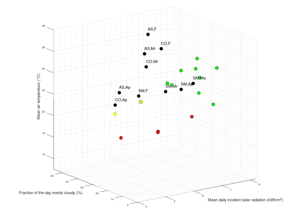
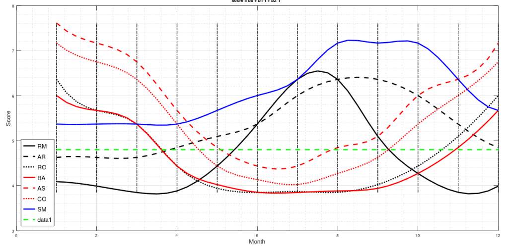
. RM = Rome; AR = Arona, Tenerife, Spain; RO = Rosario, Argentina; BA = Buenos Aires, Argentina; AS = Asunción, Paraguay; CO = Corrientes, Argentina; SM = Santa Maria, Cape Verde.

Cor. between
Y and
Spearman
(p value)
Pearson
(p value)
Pearson
corrected for t
(p value)
Pearson
corrected for R
(p value)
R0.758
(1.10e-4)
0.706
(0.509e-4)
0.204
(0.401)
Cl-0.511
(0.214e-2)
-0.583
(0.696e-3)
0.182
(0.456)
t
0.875
(4.49e-7)
0.786
(4.04e-5)
0.519
(2.27e-2)
T^40.875
(4.49e-7)
0.794
(2.85e-5)
0.515
(2.43e-2)

Table 2. Correlation coefficients (Spearman and Person) between the variables. Corrected Pearson correlations were also computed, when possible. T = mean daily absolute temperature; t = meant daily temperature in Celsius, R = mean daily solar radiation; Cl = fraction of the day mainly cloudy.

I also used the 198 data points from my previous study (Maccallini P. 2022) to test models 7 and 6 of regression. I considered the mean data on three days for all the variables (Table 3). In this case, model 6 performs better. We still have a good level of significance in the F test, and we still have a negative coefficient for t in model 7. If we use this model to make previsions on the score as a function of the month in various cities, we get Figure 3. Consider that this regression model is based on a scoring system that is slightly lower if compared with the one used for the previous analysis.

Model\beta_0\beta_1\beta_2\beta_3F test
6)\,Y=\beta_0+\beta_1 T^48.19e-15.31e-10***1.54e-6
7)\,Y=\beta_0+\beta_1 t +\beta_2 T^4-4.67e1.-9.09e-1.9.41e-9.2.14e-6

Table 3. For each regression model, I have indicated the values of the estimates of the coefficients (with their degree of significance), and the p value of the F test. The meaning of the asterisks is: . p<01, * p < 0.05; ** p<0.001; *** p = 0. T = mean daily absolute temperature; t = meant daily temperature in Celsius, R = mean daily solar radiation; Cl = fraction of the day mainly cloudy.

Figure 2. Prediction for the score by the regression model 6 of Table 3. RM = Rome; AR = Arona, Tenerife, Spain; RO = Rosario, Argentina; BA = Buenos Aires, Argentina. AS = Asunción, Paraguay; CO = Corrientes, Argentina; SM = Santa Maria, Cape Verde.

Discussion

The best regression model is Y=\beta_0+\beta_1 t +\beta_2 T^4, followed by the model \beta_0+\beta_1 T^4, and model Y=\beta_0+\beta_1 R +\beta_2 t + \beta_3 T^4. These three models have a physical meaning; namely, they express the flux of thermic energy between my body and the environment. The human body must balance the energy exchanged with the environment to maintain thermic homeostasis. The power P exchanged with the environment can be written as

(2) \,\,\,P\,=\,R+CV+CD+E

where R is the power exchange in the form of radiant energy, C is the exchange by conduction, CV is the exchange by convection, and E is the dispersion of power by evaporation. This is a simplification of complex phenomena that should also take into account the exchange of thermic power associated with the passage of atmospheric gas through the respiratory system. The power R can be further specified in the form R\,=\,K_1 R_{sun} + K_2(T_me^4-T_env^4) where K_1 R_{sun} is the power absorbed from the Sun, and the other addend is the radiant power exchanged with the environment, whit K_2 a constant that expresses radiant and geometrical properties of both my body and of the environment. While R_{sun} is radiant power in the form of short wave radiation (wavelength below 3 \mu), the other addend represents radiant power exchanged by bodies at low temperatures with a wavelength above 3 \mu (according to the Stephan-Boltzman law) (R). But what temperature is T_{env}? One first approximation might be the absolute temperature of the air, because in warm months, with the windows open, the objects surrounding us tend to acquire a superficial temperature similar to that of the air. To show that point, I analyzed the power emitted by the soil in Rome, during the year 2020, and the temperature of the air (data from ARPALAZIO). If we indicate J the daily mean power emitted per surface unit by the soil in the hemispace, the Stefan-Boltzmann law states that

(3) \,\,\,J\,=\,a\chi T_s^4

where a is a constant below 1 dependent on the material of the surface of the soil, \chi\,=\,5.6696\cdot10^{-8}\frac{W}{m^2 K^4} is the Stefan-Boltzmann constant, and T_s is the absolute temperature of the soil. If the assertion that the temperature of the soil is about the same as the temperature of the air was correct, the regression for the following linear model should have a very low p value of the F test:

(4) \,\,\,J\,=\,B_0 + B_1(273.15 + t_a)^4

And this is in fact the case, we have the regression in Figure 3, with a p value of the F test below 2.2\cdot 10^{-16}. For further details on these calculations, see (Maccallini P, 2022).

Figure 3. Linear regression between the mean daily irradiance from the Earth and the fourth power of the absolute temperature of the air (daily mean value). Data from ARPA, Rome, 2020. The analysis is described in detail in (Maccallini P, 2022).

As for the exchange of power by conduction and convection, in both cases, they are expressed by a constant multiplied by the difference in temperature between my skin and the air. That said, we can write again eq. 1 as follows:

(5) \,\,\,P\,=\,K_1 R_{sun}+K_2 (T_{skin}^4-T_{air}^4)+K_3 (t_{skin} - t_{air})

were we have removed the term linked to evaporation. In other words, the power exchanged by my body with the environment could be expressed, in first approximation, by the equation

(6) \,\,\,P\,=\,B_0+B_1 R_{sun}+B_2 t_{air} + B_3 T_{air}^4

This is model 5 of Table 1. If we consider the case of a subject who rarely leaves home, we can get rid of R_{sun} and we get model 7, the best model of regression. In a previous article, I showed that the best correlation between my status and several environmental parameters was with air temperature (R), and yet in an experiment where I simulated summer in a room with the use of a heat pump, an infrared lamp, and an air moisturizer, there was no correlation between my status and air temperature (R) (in fact the correlation had a tendency to be negative). From the perspective of this new study, I would explain the previous results as follows: in the first study performed during worm months using environmental parameters we caught the Spearman’s correlation between my status and air temperature which was a reflection of the correlation between my status and the longwave infrared radiation from the environment (proportional to the fourth power of the absolute temperature of the air); in the second study, performed during cold months within a room with artificially heated air, there was no correlation between air temperature and the infrared emission of the environment (which came from a lamp), so we found a correlation that tended to be negative perhaps because when I was feeling worse I raised the temperature of the air. It should be noted though that in models 7 and 5 the coefficient of t is negative, therefore it seems that while the longwave infrared radiation plays a positive role, the temperature of the air does not.

Conclusion

The three best regression models suggest that my improvement is linked to the thermal energy balance of the body: the lower the dispersion of radiant thermic energy, the better I feel. But at the same time, the temperature of the air has a detrimental effect. But other interpretations might be possible: there might be an effect of thermal radiation on my biology that is not linked to thermic homeostasis but instead to some other biological targets. Moreover, there might be other models of regression that I have not considered, that perform better than the ones mentioned.

Scripts

The first script is written in Octave. It calculates the regressions and their F tests (by using a custom subroutine) and it plots Figure 1 and Figure 2. It also writes the data in csv format for the second script (in R), which performs the same statistical analyses and also calculates the p values associated with each coefficient estimate.

% file name = Spot_finder_2
% date of creation = 29/01/2023 
%
close all 
clear all
#
pkg load statistics % we need this package for the F law
spline = 1 % it is one if we want a cubic spline interpolation for the last plot
#
#-------------------------------------------------------------------------------
# Data
#-------------------------------------------------------------------------------
#
months = ["Je"; "F"; "Mr"; "Ap"; "Ma"; "Jn"; "Jl"; "Au"; "S"; "O"; "N"; "D"];
%
% data of Rome (RM), Italy
%
k=1;
Spot(1,:,k) = [2,3,4.3,5.6,6.8,7.5,7.5,6.5,4.9,3.4,2.2,1.8]; % Mean daily incident solar radiation (kWh/m^2)
Spot(2,:,k) = [47,44,44,43,39,25,13,18,32,43,47,46]; % Fraction of the day mainly cloudy (%)
Spot(3,:,k) = [7,8,11,13,18,22,25,25,21,17,12,8]; % Mean air temperature (°C)
Spot(4,:,k) = [3,3,6,8,12,16,18,18,15,12,7,4]; % Min air temperature (°C)
Spot(5,:,k) = [12,13,16,19,23,27,31,31,27,22,17,13]; % Max air temperature (°C)
%
% data of Arona (AR), Tenerife, Spain
%
k=2;
Spot(1,:,k) = [3.9,4.9,6.1,7.2,7.8,8.2,8.0,7.4,6.3,5.1,4.0,3.5]; % Mean daily incident solar radiation (kWh/m^2)
Spot(2,:,k) = [32,28,26,24,21,9,2,6,21,34,38,36]; % Fraction of the day mainly cloudy (%)
Spot(3,:,k) = [19,19,19,20,21,22,24,25,25,24,22,20]; % Mean air temperature (°C)
Spot(4,:,k) = [16,16,16,17,18,20,21,22,22,21,19,17]; % Min air temperature (°C)
Spot(5,:,k) = [22,22,23,23,24,26,28,28,28,27,25,23]; % Max air temperature (°C)
%
% data of Rosario (RO), Santa Fe, Argentina
%
k=3;
Spot(1,:,k) = [7.6,6.7,5.6,4.3,3.2,2.7,3.0,3.9,5.1,6.3,7.3,7.7]; % Mean daily incident solar radiation (kWh/m^2)
Spot(2,:,k) = [28,28,28,34,45,47,44,40,36,32,30,28]; % Fraction of the day mainly cloudy (%)
Spot(3,:,k) = [25,23,22,18,14,11,10,12,15,18,21,24]; % Mean air temperature (°C)
Spot(4,:,k) = [19,18,17,13,10,7,6,7,9,13,16,18]; % Min air temperature (°C)
Spot(5,:,k) = [30,29,27,23,19,16,16,18,21,24,27,29]; % Max air temperature (°C)
%
% data of Buenos Aires (BA), Argentina
%
k=4;
Spot(1,:,k) = [7.6,6.7,5.5,4.1,3.0,2.5,2.7,3.6,4.8,6.2,7.3,7.8]; % Mean daily incident solar radiation (kWh/m^2)
Spot(2,:,k) = [29,31,31,38,48,50,48,45,41,37,33,30]; % Fraction of the day mainly cloudy (%)
Spot(3,:,k) = [24,23,22,18,15,12,11,13,14,17,20,23]; % Mean air temperature (°C)
Spot(4,:,k) = [21,20,19,15,12,9,9,10,11,14,17,19]; % Min air temperature (°C)
Spot(5,:,k) = [28,27,25,21,18,15,14,16,18,21,24,27]; % Max air temperature (°C)
%
% data of Asuncion (AS), Paraguay
%
k=5;
Spot(1,:,k) = [7.0,6.6,6.0,5.0,4.1,3.5,3.8,4.5,5.3,6.1,6.9,7.1]; % Mean daily incident solar radiation (kWh/m^2)
Spot(2,:,k) = [45,42,33,31,32,37,35,32,32,38,38,42]; % Fraction of the day mainly cloudy (%)
Spot(3,:,k) = [28,27,26,23,20,18,18,20,21,24,25,27]; % Mean air temperature (°C)
Spot(4,:,k) = [23,23,21,19,16,14,14,15,16,19,21,22]; % Min air temperature (°C)
Spot(5,:,k) = [33,32,31,28,25,23,23,25,27,29,31,32]; % Max air temperature (°C)
%
% data of Corrientes (CO), Argentina
%
k=6;
Spot(1,:,k) = [7.2,6.7,5.9,4.8,3.9,3.4,3.6,4.3,5.3,6.2,7.0,7.3]; % Mean daily incident solar radiation (kWh/m^2)
Spot(2,:,k) = [39,35,30,30,33,37,35,33,32,34,34,36,]; % Fraction of the day mainly cloudy (%)
Spot(3,:,k) = [27,26,25,22,18,16,15,17,19,22,24,26]; % Mean air temperature (°C)
Spot(4,:,k) = [22,22,20,17,14,12,11,12,14,17,19,21]; % Min air temperature (°C)
Spot(5,:,k) = [33,32,30,26,23,21,21,23,25,27,29,31]; % Max air temperature (°C)
%
% data of SantaMaria (SM), Capo Verde
%
k=7;
Spot(1,:,k) = [5.0,5.9,6.8,7.3,7.3,7.2,6.7,6.2,5.8,5.6,5.0,4.6]; % Mean daily incident solar radiation (kWh/m^2)
Spot(2,:,k) = [42,35,34,33,25,19,36,53,56,48,54,49]; % Fraction of the day mainly cloudy (%)
Spot(3,:,k) = [22,22,22,22,23,24,25,27,27,27,25,23]; % Mean air temperature (°C)
Spot(4,:,k) = [20,19,20,20,21,22,23,25,25,24,23,21]; % Min air temperature (°C)
Spot(5,:,k) = [25,25,25,26,26,27,28,30,30,30,28,26]; % Max air temperature (°C)
%
names = {"RM","AR","RO","BA","AS","CO","SM"};
types = {"-k","--k",":k","-r","--r",":r","-b","--b","-.b",}
%
for i=1:5
  max_measure(i) = max([Spot(i,:,1),Spot(i,:,2),Spot(i,:,3),Spot(i,:,4),Spot(i,:,5),Spot(i,:,6),Spot(i,:,7)])
endfor
%
%-------------------------------------------------------------------------------
% Subroutine for F-test
%-------------------------------------------------------------------------------
%
function [pval,R2,TS] = F_test (M,b,beta)
  r = length(M(1,:))-1; % number of explanatory variables
  n = length(M(:,1)) % number of data points
  R = b-M*beta; % residues
  SSR = 0;
  Sbb = 0;
  for i=1:n
    SSR = SSR + R(i)^2; % sum of squared residues
    Sbb = Sbb + b(i)^2;
  endfor
  Sbb = Sbb - n*(mean(b))^2;
  R2 = (Sbb - SSR)/Sbb; % R squared
  TS = R2*(n-r-1)/(r*(1-R2)); % test statistics
  pval = 1 - fcdf(TS,r,n-r-1); % F-test
endfunction
%
%-------------------------------------------------------------------------------
% Subroutine plot_score
%-------------------------------------------------------------------------------
%
function Plot_score (score, h, model, names, types, spline)
    figure(5) % Plotting of the Scoring for the query spots
    %
    for k=1:length(names)
      if (spline==1)
        yi = interp1([1:1:12],score(:,k),[1:0.25:12],"spline")
        plot([1:0.25:12],yi,char(types{k}),"linewidth",1.5)
        hold on
      else
        plot([1:1:12],score(:,k),char(types{k}),"linewidth",1.5)
        hold on
      endif
    endfor
    plot([1,12],[5,5],"--g","linewidth",1.5)
    title(model{h})
    legend(char(names{1:length(names)}),"location","southwest",'fontsize',15)
    xlabel("Month",'fontsize',15);
    ylabel("Score",'fontsize',15);
    grid on
    grid minor on
endfunction
%
%-------------------------------------------------------------------------------
figure 1 % mean temp, irradiation, cloudiness with storing of data for regressions
%-------------------------------------------------------------------------------
%
% plotting Rome
%
k=1;
n=1;
for i=1:12
  if (and(i>=6,i<9))
    plot3(Spot(1,i,k),Spot(2,i,k),Spot(3,i,k),'o','markersize',6,'markerfacecolor','g','markeredgecolor','k')
    b(n)=6;
    M(n,1:4)=[1,Spot(1,i,k),Spot(2,i,k),Spot(3,i,k)];
    n=n+1
  endif
  if (or(i<6,i>9))
    plot3(Spot(1,i,k),Spot(2,i,k),Spot(3,i,k),'o','markersize',6,'markerfacecolor','r','markeredgecolor','k')
  endif
  if (or(and(i>3,i<5),i>9))
    b(n)=4;
    M(n,1:4)=[1,Spot(1,i,k),Spot(2,i,k),Spot(3,i,k)];
    n=n+1
  endif
  if (i==5)
    b(n)=5;
    M(n,1:4)=[1,Spot(1,i,k),Spot(2,i,k),Spot(3,i,k)];
    n=n+1
  endif
  if (i==9)
    plot3(Spot(1,i,k),Spot(2,i,k),Spot(3,i,k),'o','markersize',6,'markerfacecolor','y','markeredgecolor','g')
    b(n)=5.7;
    M(n,1:4)=[1,Spot(1,i,k),Spot(2,i,k),Spot(3,i,k)];
    n=n+1
  endif
  hold on
endfor
%
% plotting Arona
%
k=2;
for i=1:12
  if (i==5)
    plot3(Spot(1,i,k),Spot(2,i,k),Spot(3,i,k),'o','markersize',6,'markerfacecolor','g','markeredgecolor','k')
    b(n)=6
    M(n,1:4)=[1,Spot(1,i,k),Spot(2,i,k),Spot(3,i,k)];
    n=n+1
  endif
  if (and(i>=1,i<5))
    plot3(Spot(1,i,k),Spot(2,i,k),Spot(3,i,k),'o','markersize',6,'markerfacecolor','r','markeredgecolor','k')
    b(n)=4
    M(n,1:4)=[1,Spot(1,i,k),Spot(2,i,k),Spot(3,i,k)];
    n=n+1
  endif
    hold on
endfor
%
% plotting Rosario
%
k=3;
for i=1:12
  if (and(i>=1,i<3))
    plot3(Spot(1,i,k),Spot(2,i,k),Spot(3,i,k),'o','markersize',6,'markerfacecolor','g','markeredgecolor','k')
    b(n)=6
    M(n,1:4)=[1,Spot(1,i,k),Spot(2,i,k),Spot(3,i,k)];
    n=n+1
  endif
  if (i==3)
    plot3(Spot(1,i,k),Spot(2,i,k),Spot(3,i,k),'o','markersize',6,'markerfacecolor','y','markeredgecolor','k')
    b(n)=5.5
    M(n,1:4)=[1,Spot(1,i,k),Spot(2,i,k),Spot(3,i,k)];
    n=n+1
  endif
  hold on
endfor
%
% plotting CABA
%
k=4;
for i=1:12
  if (or(i==12,i==1,i==2))
    plot3(Spot(1,i,k),Spot(2,i,k),Spot(3,i,k),'o','markersize',6,'markerfacecolor','g','markeredgecolor','k')
    b(n)=6
    M(n,1:4)=[1,Spot(1,i,k),Spot(2,i,k),Spot(3,i,k)];
    n=n+1
  endif
  if (i<12)
    hold on
  endif
endfor
%
% plotting query spots
%
% Asuncion
%
k=5;
for i=2:4
  plot3(Spot(1,i,k),Spot(2,i,k),Spot(3,i,k),'o','markersize',6,'markerfacecolor','k','markeredgecolor','k')
  text(Spot(1,i,k),Spot(2,i,k),Spot(3,i,k)+0.5, strcat(char(names{k}),", ",months(i,:)),'fontsize',15)
endfor
%
% Corrientes
%
k=6;
for i=2:4
  plot3(Spot(1,i,k),Spot(2,i,k),Spot(3,i,k),'o','markersize',6,'markerfacecolor','k','markeredgecolor','k')
  text(Spot(1,i,k),Spot(2,i,k),Spot(3,i,k)+0.5, strcat(char(names{k}),", ",months(i,:)),'fontsize',15)
endfor
%
% Santa Maria
%
k=7;
for i=2:5
  plot3(Spot(1,i,k),Spot(2,i,k),Spot(3,i,k),'o','markersize',6,'markerfacecolor','k','markeredgecolor','k')
  text(Spot(1,i,k),Spot(2,i,k),Spot(3,i,k)+0.5, strcat(char(names{k}),", ",months(i,:)),'fontsize',15)
endfor
%
grid on
grid minor on
xlabel("Mean daily incident solar radiation (kWh/m^{2})",'fontsize',15);
ylabel("Fraction of the day mainly cloudy (%)",'fontsize',15);
zlabel("Mean air temperature (°C)",'fontsize',15);
axis ('square')
axis([4,max_measure(1),0,max_measure(2),15,max_measure(3)])
%
%-------------------------------------------------------------------------------
% Regressions
%-------------------------------------------------------------------------------
%
n=n-1; % number of measures
%
b = transpose(b)
x = cell() % it contains the coefficients of the models
model = cell() % it contains the description of the models
matrix = cell() % it contains the matrix of the regression
k = 0;
%
for i=1:n
  A(i,1:3)=[1,M(i,2),M(i,4)]
endfor
k = k+1;
[x{k}, std, mse, S] = lscov (A, b)
[pval(k), R2(k), TS(k)] = F_test (A, b, x{k})
model{k} = "socre = b0 + b1*Rad + b2*t"
matrix{k} = A;
clear A
%
for i=1:n
  A(i,1:3)=[1,M(i,3),M(i,4)]
endfor
k = k+1;
[x{k}, std, mse, S] = lscov (A, b)
[pval(k), R2(k), TS(k)] = F_test (A, b, x{k})
model{k} = "socre = b0 + b1*Cl + b2*t"
matrix{k} = A;
clear A
%
for i=1:n
  A(i,1:4)=[1,M(i,2),M(i,3),M(i,4)]
endfor
k = k+1;
[x{k}, std, mse, S] = lscov (A, b)
[pval(k), R2(k), TS(k)] = F_test (A, b, x{k})
model{k} = "socre = b0 + b1*Rad + b1*Cl + b2*t"
matrix{k} = A;
clear A
%
for i=1:n
  A(i,1:3)=[1,M(i,2),(273.15+M(i,4))^4]
endfor
k = k+1;
[x{k}, std, mse, S] = lscov (A, b)
[pval(k), R2(k), TS(k)] = F_test (A, b, x{k})
model{k} = "socre = b0 + b1*Rad + b2*T^{4}"
matrix{k} = A;
clear A
%
for i=1:n
  A(i,1:4)=[1,M(i,2),M(i,4),(273.15+M(i,4))^4]
endfor
k = k+1;
[x{k}, std, mse, S] = lscov (A, b)
[pval(k), R2(k), TS(k)] = F_test (A, b, x{k})
model{k} = "socre = b0 + b1*Rad + b2*t + b3*T^{4}"
matrix{k} = A;
clear A
%
for i=1:n
  A(i,1:2)=[1,(273.15+M(i,4))^4]
endfor
k = k+1;
[x{k}, std, mse, S] = lscov (A, b)
[pval(k), R2(k), TS(k)] = F_test (A, b, x{k})
model{k} = "socre = b0 + b1*T^{4}"
matrix{k} = A;
clear A
%
for i=1:n
  A(i,1:3)=[1,M(i,4),(273.15+M(i,4))^4]
endfor
k = k+1;
[x{k}, std, mse, S] = lscov (A, b)
[pval(k), R2(k), TS(k)] = F_test (A, b, x{k})
model{k} = "socre = b0 + b1*t + b2*T^{4}"
matrix{k} = A;
clear A
%
%-------------------------------------------------------------------------------
% Selection of the best model
%-------------------------------------------------------------------------------
%
for i=1:length(pval)
  if (pval(i)==min(pval))
    best=i;
  endif
endfor
%
%-------------------------------------------------------------------------------
% Region of the plane Rad-Temp with high score according to the regression
% model
%-------------------------------------------------------------------------------
%
R(1)= 4;
R(2)= max_measure(1);
Temp_R(1) = ( 5.5 - x{1}(1) - x{1}(2)*R(1) )/x{1}(3);
Temp_R(2) = ( 5.5 - x{1}(1) - x{1}(2)*R(2) )/x{1}(3);
%
%-------------------------------------------------------------------------------
% Region of the plane Cloudiness-Temp with high score according to the regression
% model
%-------------------------------------------------------------------------------
%
Cl(1)= 0;
Cl(2)= max_measure(2);
Temp_Cl(1) = ( 5.5 - x{2}(1) - x{2}(2)*Cl(1) )/x{2}(3);
Temp_Cl(2) = ( 5.5 - x{2}(1) - x{2}(2)*Cl(2) )/x{2}(3);
%
%-------------------------------------------------------------------------------
figure 2 % mean temp and irradiation
%-------------------------------------------------------------------------------
%
% plotting Rome
%
k=1;
for i=1:12
  if (and(i>=6,i<9))
    plot(Spot(1,i,k),Spot(3,i,k),'o','markersize',6,'markerfacecolor','g','markeredgecolor','k')
  endif
  if (or(i<6,i>9))
    plot(Spot(1,i,k),Spot(3,i,k),'o','markersize',6,'markerfacecolor','r','markeredgecolor','k')
  endif
  if (i==9)
    plot(Spot(1,i,k),Spot(3,i,k),'o','markersize',6,'markerfacecolor','y','markeredgecolor','g')
  endif
  hold on
endfor
%
% plotting Arona
%
k=2;
for i=1:12
  if (i==5)
    plot(Spot(1,i,k),Spot(3,i,k),'o','markersize',6,'markerfacecolor','g','markeredgecolor','k')
  endif
  if (and(i>=1,i<5))
    plot(Spot(1,i,k),Spot(3,i,k),'o','markersize',6,'markerfacecolor','r','markeredgecolor','k')
  endif
    hold on
endfor
%
% plotting Rosario
%
k=3;
for i=1:12
  if (and(i>=1,i<3))
    plot(Spot(1,i,k),Spot(3,i,k),'o','markersize',6,'markerfacecolor','g','markeredgecolor','k')
  endif
  if (i==3)
    plot(Spot(1,i,k),Spot(3,i,k),'o','markersize',6,'markerfacecolor','y','markeredgecolor','k')
  endif
  hold on
endfor
%
% plotting CABA
%
k=4;
for i=1:12
  if (or(i==12,i==1,i==2))
    plot(Spot(1,i,k),Spot(3,i,k),'o','markersize',6,'markerfacecolor','g','markeredgecolor','k')
  endif
  if (i<12)
    hold on
  endif
endfor
%
% plotting query spots
%
% Asuncion
%
k=5;
for i=2:4
  plot(Spot(1,i,k),Spot(3,i,k),'o','markersize',6,'markerfacecolor','k','markeredgecolor','k')
  text(Spot(1,i,k),Spot(3,i,k)+0.5, strcat(char(names{k}),", ",months(i,:)),'fontsize',15)
endfor
%
% Corrientes
%
k=6;
for i=2:4
  plot(Spot(1,i,k),Spot(3,i,k),'o','markersize',6,'markerfacecolor','k','markeredgecolor','k')
  text(Spot(1,i,k),Spot(3,i,k)+0.5, strcat(char(names{k}),", ",months(i,:)),'fontsize',15)
endfor
%
% Santa Maria
%
k=7;
for i=3:5
  plot(Spot(1,i,k),Spot(3,i,k),'o','markersize',6,'markerfacecolor','k','markeredgecolor','k')
  text(Spot(1,i,k),Spot(3,i,k)+0.5, strcat(char(names{k}),", ",months(i,:)),'fontsize',15)
endfor
%
plot([R(1),R(2)],[Temp_R(1),Temp_R(2)],"--k","linewidth",1)
%
grid on
grid minor on
xlabel("Mean daily incident solar radiation (kWh/m^{2})",'fontsize',15);
ylabel("Mean air temperature (°C)",'fontsize',15);
axis([R(1),R(2),15,max_measure(3)])
%
%-------------------------------------------------------------------------------
figure 3 % mean temp and cloudiness
%-------------------------------------------------------------------------------
%
% plotting Rome
%
k=1;
for i=1:12
  if (and(i>=6,i<9))
    plot(Spot(2,i,k),Spot(3,i,k),'o','markersize',6,'markerfacecolor','g','markeredgecolor','k')
  endif
  if (or(i<6,i>9))
    plot(Spot(2,i,k),Spot(3,i,k),'o','markersize',6,'markerfacecolor','r','markeredgecolor','k')
  endif
  if (i==9)
    plot(Spot(2,i,k),Spot(3,i,k),'o','markersize',6,'markerfacecolor','y','markeredgecolor','g')
  endif
  hold on
endfor
%
% plotting Arona
%
k=2;
for i=1:12
  if (i==5)
    plot(Spot(2,i,k),Spot(3,i,k),'o','markersize',6,'markerfacecolor','g','markeredgecolor','k')
  endif
  if (and(i>=1,i<5))
    plot(Spot(2,i,k),Spot(3,i,k),'o','markersize',6,'markerfacecolor','r','markeredgecolor','k')
  endif
    hold on
endfor
%
% plotting Rosario
%
k=3;
for i=1:12
  if (and(i>=1,i<3))
    plot(Spot(2,i,k),Spot(3,i,k),'o','markersize',6,'markerfacecolor','g','markeredgecolor','k')
  endif
  if (i==3)
    plot(Spot(2,i,k),Spot(3,i,k),'o','markersize',6,'markerfacecolor','y','markeredgecolor','k')
  endif
  hold on
endfor
%
% plotting CABA
%
k=4;
for i=1:12
  if (or(i==12,i==1,i==2))
    plot(Spot(2,i,k),Spot(3,i,k),'o','markersize',6,'markerfacecolor','g','markeredgecolor','k')
  endif
  if (i<12)
    hold on
  endif
endfor
%
% plotting query spots
%
% Buenos Aires
%
i=2;
k=4;
plot(Spot(2,i,k),Spot(3,i,k),'o','markersize',6,'markerfacecolor','k','markeredgecolor','k')
text(Spot(2,i,k),Spot(3,i,k)-0.5, strcat(char(names{k}),", ",months(i,:)),'fontsize',15)
%
% Asuncion
%
k=5;
for i=2:4
  plot(Spot(2,i,k),Spot(3,i,k),'o','markersize',6,'markerfacecolor','k','markeredgecolor','k')
  text(Spot(2,i,k),Spot(3,i,k)+0.5, strcat(char(names{k}),", ",months(i,:)),'fontsize',15)
endfor
%
% Corrientes
%
k=6;
for i=2:4
  plot(Spot(2,i,k),Spot(3,i,k),'o','markersize',6,'markerfacecolor','k','markeredgecolor','k')
  text(Spot(2,i,k),Spot(3,i,k)-0.5, strcat(char(names{k}),", ",months(i,:)),'fontsize',15)
endfor
%
% Santa Maria
%
k=7;
for i=3:5
  plot(Spot(2,i,k),Spot(3,i,k),'o','markersize',6,'markerfacecolor','k','markeredgecolor','k')
  text(Spot(2,i,k),Spot(3,i,k)+0.5, strcat(char(names{k}),", ",months(i,:)),'fontsize',15)
endfor
%
plot([Cl(1),Cl(2)],[Temp_Cl(1),Temp_Cl(2)],"--k","linewidth",1)
%
grid on
grid minor on
xlabel("Fraction of the day mainly cloudy (%)",'fontsize',15);
ylabel("Mean air temperature (°C)",'fontsize',15);
axis([Cl(1),Cl(2),15,max_measure(3)])
%
%-------------------------------------------------------------------------------
% Plotting the scoring for each city according to the best model
%-------------------------------------------------------------------------------
%
switch best
  case 1
    %
    % Scoring for the query spots according to model h
    %
    h=1;
    for i=1:12
      for k=1:length(names)
        score(i,k) = x{h}(1)+x{h}(2)*Spot(1,i,k)+x{h}(3)*Spot(3,i,k);
      endfor
    endfor
    %
    figure(5) % Plotting of the Scoring for the query spots
    %
    for k=1:length(names)
      plot([1:1:12],score(:,k),char(types{k}),"linewidth",1.5)
      hold on
    endfor
    plot([1,12],[5,5],"--g","linewidth",1.5)
    title(model{h},'fontsize',15)
    legend(char(names{1:length(names)}),"location","southwest",'fontsize',15)
    xlabel("Month",'fontsize',15);
    ylabel("Score",'fontsize',15);
    grid on
    grid minor on
  case 2
    %
    % Scoring for the query spots according to model h 
    %
    h=2;
    for i=1:12
      for k=1:length(names)
        score(i,k) = x{h}(1)+x{h}(2)*Spot(2,i,k)+x{h}(3)*Spot(3,i,k);
      endfor
    endfor
    %
    figure(5) % Plotting of the Scoring for the query spots
    %
    for k=1:length(names)
      plot([1:1:12],score(:,k),char(types{k}),"linewidth",1.5)
      hold on
    endfor
    plot([1,12],[5,5],"--g","linewidth",1.5)
    title(model{h},'fontsize',15)
    legend(char(names{1:length(names)}),"location","southwest",'fontsize',15)
    xlabel("Month",'fontsize',15);
    ylabel("Score",'fontsize',15);
    grid on
    grid minor on
  case 3
    %
    % Scoring for the query spots according to model h
    %
    h=3;
    for i=1:12
      for k=1:length(names)
        score(i,k) = x{h}(1)+x{h}(2)*Spot(1,i,k)+x{h}(3)*Spot(2,i,k)+x{h}(4)*Spot(3,i,k);
      endfor
    endfor
    %
    figure(5) % Plotting of the Scoring for the query spots
    %
    for k=1:length(names)
      plot([1:1:12],score(:,k),char(types{k}),"linewidth",1.5)
      hold on
    endfor
    plot([1,12],[5,5],"--g","linewidth",1.5)
    title(model{h},'fontsize',15)
    legend(char(names{1:length(names)}),"location","southwest",'fontsize',15)
    xlabel("Month",'fontsize',15);
    ylabel("Score",'fontsize',15);
    grid on
    grid minor on
  case 4
    %
    % Scoring for the query spots according to model h
    %
    h=4;
    for i=1:12
      for k=1:length(names)
        score(i,k) = x{h}(1)+x{h}(2)*Spot(1,i,k)+x{h}(3)*(Spot(3,i,k)^4);
      endfor
    endfor
    %
    figure(5) % Plotting of the Scoring for the query spots
    %
    for k=1:length(names)
      plot([1:1:12],score(:,k),char(types{k}),"linewidth",1.5)
      hold on
    endfor
    plot([1,12],[5,5],"--g","linewidth",1.5)
    title(model{h},'fontsize',15)
    legend(char(names{1:length(names)}),"location","southwest",'fontsize',15)
    xlabel("Month",'fontsize',15);
    ylabel("Score",'fontsize',15);
    grid on
    grid minor on
  case 5
    %
    % Scoring for the query spots according to model h
    %
    h=5;
    for i=1:12
      for k=1:length(names)
        score(i,k) = x{h}(1)+x{h}(2)*Spot(1,i,k)+x{h}(3)*Spot(3,i,k)+x{h}(4)*(Spot(3,i,k)^4);
      endfor
    endfor
    %
    figure(5) % Plotting of the Scoring for the query spots
    %
    for k=1:length(names)
      plot([1:1:12],score(:,k),char(types{k}),"linewidth",1.5)
      hold on
    endfor
    plot([1,12],[5,5],"--g","linewidth",1.5)
    title(model{h},'fontsize',15)
    legend(char(names{1:length(names)}),"location","southwest",'fontsize',15)
    xlabel("Month",'fontsize',15);
    ylabel("Score",'fontsize',15);
    grid on
    grid minor on
  case 6
    %
    % Scoring for the query spots according to model h
    %
    h=6;
    for i=1:12
      for k=1:length(names)
        score(i,k) = x{h}(1)+x{h}(2)*((273.15+Spot(3,i,k))^4);
      endfor
    endfor
    %
    Plot_score (score, h, model, names, types, spline)
  case 7
    %
    % Scoring for the query spots according to model h
    %
    h=7;
    for i=1:12
      for k=1:length(names)
        score(i,k) = x{h}(1)+x{h}(2)*Spot(3,i,k)+x{h}(3)*((273.15+Spot(3,i,k))^4);
      endfor
    endfor
    %
    Plot_score (score, h, model, names, types, spline)
endswitch
%
%-------------------------------------------------------------------------------
% We save the data for the regressions
%-------------------------------------------------------------------------------
%
save("M.csv","M")
save("Y.csv","b")
# file name: spot_finder
#
# Asunciòn, 9 marzo 2023
#
#-------------------------------------------------------------------------------
# This script performs the linear regressions performed also by the Octave script
# that goes under the same name
#-------------------------------------------------------------------------------
#
library(ppcor) # we need this for the partial correlation analysis
#
#-------------------------------------------------------------------------------
# Data 
#-------------------------------------------------------------------------------
#
Y<-read.csv(file = "Y.csv", header = F, sep =" ", comment.char = "#") # the response variable
Y<-Y[,2]
M<-read.csv(file = "M.csv", header = F, sep =" ", comment.char = "#")
M<-M[,2:5]
colnames(M)<-c("unity","Rad","Cl","meanT")
AT<-273.15+M$meanT # absolute temperature
#
#-------------------------------------------------------------------------------
# Regression (model x1 + x2*R + x3*t) 
#-------------------------------------------------------------------------------
#
R_t_re<-lm(Y~M$Rad+M$meanT)
summary(R_t_re)
#
#-------------------------------------------------------------------------------
# Regression (model x1 + x2*Cl + x3*t) 
#-------------------------------------------------------------------------------
#
C_t_re<-lm(Y~M$Cl+M$meanT)
summary(C_t_re)
#
#-------------------------------------------------------------------------------
# Regression (model x1 + x2*R + x3*Cl + x4*t) 
#-------------------------------------------------------------------------------
#
R_C_t_re<-lm(Y~M$Rad+M$Cl+M$meanT)
summary(R_C_t_re)
#
#-------------------------------------------------------------------------------
# Regression (model x1 + x2*R + x4*T^4) 
#-------------------------------------------------------------------------------
#

R_T4_re<-lm(Y~M$Rad+I(AT^4))
summary(R_T4_re)
#
#-------------------------------------------------------------------------------
# Regression (model x1 + x2*R + x3*t + x4*T^4) 
#-------------------------------------------------------------------------------
#
R_t_T4_re<-lm(Y~M$Rad+M$meanT+I(AT^4))
summary(R_t_T4_re)
#
#-------------------------------------------------------------------------------
# Regression (model x1 + x2*T^4) 
#-------------------------------------------------------------------------------
#
T4_re<-lm(Y~I(AT^4))
summary(T4_re)
#
#-------------------------------------------------------------------------------
# Regression (model x1 + x2*t + x3T^4) 
#-------------------------------------------------------------------------------
#
t_T4_re<-lm(Y~M$meanT+I(AT^4))
summary(t_T4_re)
#
#-------------------------------------------------------------------------------
# Spearman coefficients and corresponding p values
#-------------------------------------------------------------------------------
#
Spearman_Rad<-cor.test(Y,M$Rad,alternative="two.sided",method="spearman",conf.level=0.95)
Spearman_Rad
Spearman_Cl<-cor.test(Y,M$Cl,alternative="two.sided",method="spearman",conf.level=0.95)
Spearman_Cl
Spearman_meanT<-cor.test(Y,M$meanT,alternative="two.sided",method="spearman",conf.level=0.95)
Spearman_meanT
#
#-------------------------------------------------------------------------------
# Pearson coefficients, corresponding p values, and partial correlations
#-------------------------------------------------------------------------------
#
Ro_Y_R<-cor.test(Y,M$Rad,alternative="two.sided",method="pearson",conf.level=0.95)
Ro_Y_R
Ro_Y_C<-cor.test(Y,M$Cl,alternative="two.sided",method="pearson",conf.level=0.95)
Ro_Y_C
Ro_Y_t<-cor.test(Y,M$meanT,alternative="two.sided",method="pearson",conf.level=0.95)
Ro_Y_t
Ro_Y_T4<-cor.test(Y,I(AT^4),alternative="two.sided",method="pearson",conf.level=0.95)
Ro_Y_T4
#
Ro_Y_R_t<-pcor.test(Y,M$Rad,M$meanT,method="pearson")
Ro_Y_R_t
Ro_Y_R_T4<-pcor.test(Y,M$Rad,I(AT^4),method="pearson")
Ro_Y_R_T4
Ro_Y_C_t<-pcor.test(Y,M$Cl,M$meanT,method="pearson")
Ro_Y_C_t
Ro_Y_C_T4<-pcor.test(Y,M$Cl,I(AT^4),method="pearson")
Ro_Y_C_T4
Ro_Y_t_R<-pcor.test(Y,M$meanT,M$Rad,method="pearson")
Ro_Y_t_R
Ro_Y_T4_R<-pcor.test(Y,I(AT^4),M$Rad,method="pearson")
Ro_Y_T4_R
Ro_Y_T4_T<-pcor.test(Y,I(AT^4),M$meanT,method="pearson")
Ro_Y_T4_T
#
#-------------------------------------------------------------------------------
# Data of the first environmental study
#-------------------------------------------------------------------------------
#
mydata<-read.csv(file = "correlation.csv", header = T, sep =";")
#
attach(mydata)
n<-length(Station)
Y<-c()
for (i in 1:n) Y[i]<-mean(c(Score1[i], Score2[i], Score3[i]), na.rm = T )
meanT<-Tempmean
meanP<-c()
for (i in 1:n) meanP[i]<-mean(c(Pressuremax[i],Pressuremin[i]), na.rm = T)
meanRH<-RHmean
#
#-------------------------------------------------------------------------------
# mean values
#-------------------------------------------------------------------------------
#
d<-3 # mean on d days
for (i in 1:(n-d)) {
  meanT[i]<-mean(meanT[i:(i+d)], na.rm = T)
  meanP[i]<-mean(meanP[i:(i+d)], na.rm = T)
  meanRH[i]<-mean(meanRH[i:(i+d)], na.rm = T)
  Y[i]<-mean(Y[i:(i+d)], na.rm = T)
}
AT<-273.15+meanT
#
#-------------------------------------------------------------------------------
# Regression (model x1 + x2*T^4) 
#-------------------------------------------------------------------------------
#
T4_re<-lm(Y~I(AT^4))
summary(T4_re)
#
#-------------------------------------------------------------------------------
# Regression (model x1 + x2*t + x3T^4) 
#-------------------------------------------------------------------------------
#
t_T4_re<-lm(Y~meanT+I(AT^4))
summary(t_T4_re)